Weierstrass zeta function
(0.006 seconds)
1—10 of 23 matching pages
1: 23.1 Special Notation
…
►The main functions treated in this chapter are the Weierstrass
-function
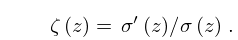
; the Weierstrass zeta function
; the Weierstrass sigma function
; the elliptic modular function
; Klein’s complete invariant ; Dedekind’s eta function
.
…
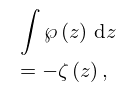
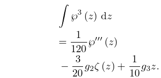
2: 23.14 Integrals
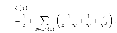
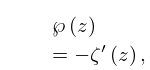
3: 23.2 Definitions and Periodic Properties
…
►
23.2.5
…
►
23.2.7
►
23.2.8
►
and are meromorphic functions with poles at the lattice points.
…
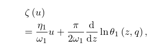
►The function
is quasi-periodic: for ,
…
4: 25.1 Special Notation
…
►The main related functions are the Hurwitz zeta function
, the dilogarithm , the polylogarithm (also known as Jonquière’s function
), Lerch’s transcendent , and the Dirichlet -functions
.
5: 23.3 Differential Equations
…
►As functions of and , and are meromorphic and is entire.
…
6: 23.4 Graphics
…
►Line graphs of the Weierstrass functions
, , and , illustrating the lemniscatic and equianharmonic cases.
…
►Surfaces for the Weierstrass functions
, , and .
…
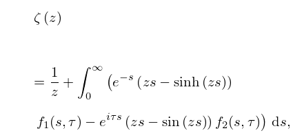
7: 23.11 Integral Representations
…
►
23.11.3
…
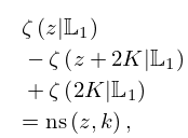
8: 23.6 Relations to Other Functions
…
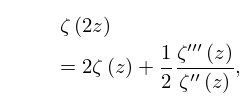
►
23.6.13
…
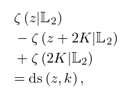
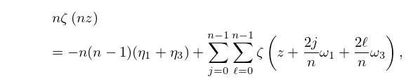
►
23.6.27
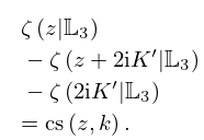
►
23.6.28
►
23.6.29
…
►For representations of general elliptic functions (§23.2(iii)) in terms of and see Lawden (1989, §§8.9, 8.10), and for expansions in terms of see Lawden (1989, §8.11).
…
