Weber%E2%80%93Schafheitlin%20discontinuous%20integrals

SearchAdvancedHelp

(0.005 seconds)

1—10 of 508 matching pages

1: 11.10 Anger–Weber Functions

§11.10 Anger–Weber Functions

►

§11.10(i) Definitions

… ►

§11.10(v) Interrelations

… ► … ►

§11.10(x) Integrals and Sums

…

2: 1.14 Integral Transforms

§1.14 Integral Transforms

… ►where the last integral denotes the Cauchy principal value (1.4.25). … ►If $f(t)$ and $f^{\prime }(t)$ are piecewise continuous on $[0,\mathrm{\infty })$ with discontinuities at ($0=$) , then … ►

§1.14(viii) Compendia

►For more extensive tables of the integral transforms of this section and tables of other integral transforms, see Erdélyi et al. (1954a, b), Gradshteyn and Ryzhik (2000), Marichev (1983), Oberhettinger (1972, 1974, 1990), Oberhettinger and Badii (1973), Oberhettinger and Higgins (1961), Prudnikov et al. (1986a, b, 1990, 1992a, 1992b).

3: 10.75 Tables

… ►

Bickley et al. (1952) tabulates $J_n\left(x\right)$, $Y_n\left(x\right)$ or $x^n{Y}_n\left(x\right)$, $n=2(1)20$, $x=0$($.01$ or $.1$) $10(.1)25$, 8D (for $J_n\left(x\right)$), 8S (for $Y_n\left(x\right)$ or $x^n{Y}_n\left(x\right)$); $J_n\left(x\right)$, $Y_n\left(x\right)$, $n=0(1)20$, $x=0$ or $0.1(.1)25$, 10D (for $J_n\left(x\right)$), 10S (for $Y_n\left(x\right)$).

… ►

The main tables in Abramowitz and Stegun (1964, Chapter 9) give $J_0\left(x\right)$ to 15D, $J_1\left(x\right)$, $J_2\left(x\right)$, $Y_0\left(x\right)$, $Y_1\left(x\right)$ to 10D, $Y_2\left(x\right)$ to 8D, $x=0(.1)17.5$; $Y_n\left(x\right)-(2/\pi )J_n\left(x\right)\ln x$, $n=0,1$, $x=0(.1)2$, 8D; $J_n\left(x\right)$, $Y_n\left(x\right)$, $n=3(1)9$, $x=0(.2)20$, 5D or 5S; $J_n\left(x\right)$, $Y_n\left(x\right)$, $n=0(1)20(10)50,100$, $x=1,2,5,10,50,100$, 10S; modulus and phase functions $\sqrt{x}{M}_n\left(x\right)$, ${\theta }_n\left(x\right)-x$, $n=0,1,2$, $1/x=0(.01)0.1$, 8D.

►

Achenbach (1986) tabulates $J_0\left(x\right)$, $J_1\left(x\right)$, $Y_0\left(x\right)$, $Y_1\left(x\right)$, $x=0(.1)8$, 20D or 18–20S.

… ►

Olver (1960) tabulates $j_{n,m}$, $J_n^{\prime }\left(j_{n,m}\right)$, $j_{n,m}^{\prime }$, $J_n\left(j_{n,m}^{\prime }\right)$, $y_{n,m}$, $Y_n^{\prime }\left(y_{n,m}\right)$, $y_{n,m}^{\prime }$, $Y_n\left(y_{n,m}^{\prime }\right)$, $n=0(\frac{1}{2})20⁤\frac{1}{2}$, $m=1(1)50$, 8D. Also included are tables of the coefficients in the uniform asymptotic expansions of these zeros and associated values as $n\to \mathrm{\infty }$; see §10.21(viii), and more fully Olver (1954).

… ►

Abramowitz and Stegun (1964, Chapter 9) tabulates $j_{n,m}$, $J_n^{\prime }\left(j_{n,m}\right)$, $j_{n,m}^{\prime }$, $J_n\left(j_{n,m}^{\prime }\right)$, $n=0(1)8$, $m=1(1)20$, 5D (10D for $n=0$), $y_{n,m}$, $Y_n^{\prime }\left(y_{n,m}\right)$, $y_{n,m}^{\prime }$, $Y_n\left(y_{n,m}^{\prime }\right)$, $n=0(1)8$, $m=1(1)20$, 5D (8D for $n=0$), $J_0\left(j_{0,m}x\right)$, $m=1(1)5$, $x=0(.02)1$, 5D. Also included are the first 5 zeros of the functions $x{J}_1\left(x\right)-\lambda J_0\left(x\right)$, $J_1\left(x\right)-\lambda x{J}_0\left(x\right)$, $J_0\left(x\right)Y_0\left(\lambda x\right)-Y_0\left(x\right)J_0\left(\lambda x\right)$, $J_1\left(x\right)Y_1\left(\lambda x\right)-Y_1\left(x\right)J_1\left(\lambda x\right)$, $J_1\left(x\right)Y_0\left(\lambda x\right)-Y_1\left(x\right)J_0\left(\lambda x\right)$ for various values of $\lambda$ and ${\lambda }^{-1}$ in the interval $[0,1]$, 4–8D.

…

4: 11.14 Tables

… ►

Abramowitz and Stegun (1964, Chapter 12) tabulates ${\int }_0^x(I_0\left(t\right)-{𝐋}_0\left(t\right))dt$ and $(2/\pi ){\int }_x^{\mathrm{\infty }}{t}^{-1}{𝐇}_0\left(t\right)dt$ for $x=0(.1)5$ to 5D or 7D; ${\int }_0^x({𝐇}_0\left(t\right)-Y_0\left(t\right))dt-(2/\pi )\ln x$, ${\int }_0^x(I_0\left(t\right)-{𝐋}_0\left(t\right))dt-(2/\pi )\ln x$, and ${\int }_x^{\mathrm{\infty }}{t}^{-1}({𝐇}_0\left(t\right)-Y_0\left(t\right))dt$ for $x^{-1}=0(.01)0.2$ to 6D.

… ►

§11.14(iv) Anger–Weber Functions

►

Bernard and Ishimaru (1962) tabulates ${𝐉}_{\nu }\left(x\right)$ and ${𝐄}_{\nu }\left(x\right)$ for $\nu =-10(.1)10$ and $x=0(.1)10$ to 5D.

►

Jahnke and Emde (1945) tabulates ${𝐄}_n\left(x\right)$ for $n=1,2$ and $x=0(.01)14.99$ to 4D.

►

§11.14(v) Incomplete Functions

…

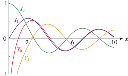
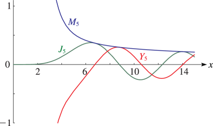
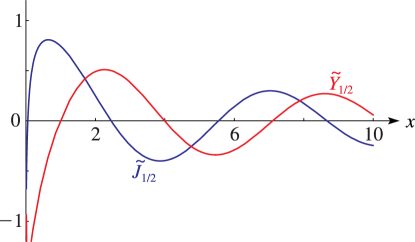
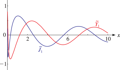
5: 10.3 Graphics

… ►

►►

Figure 10.3.1: $J_0\left(x\right)$, $Y_0\left(x\right)$, $J_1\left(x\right)$, $Y_1\left(x\right)$, $0\le x\le 10$. Magnify

►

►►

Figure 10.3.2: $J_5\left(x\right)$, $Y_5\left(x\right)$, $M_5\left(x\right)$, $0\le x\le 15$. Magnify

… ►

►►

Figure 10.3.17: ${\tilde{J}}_{1/2}\left(x\right)$, ${\tilde{Y}}_{1/2}\left(x\right)$, $0.01\le x\le 10$. Magnify

►

►►

Figure 10.3.18: ${\tilde{J}}_1\left(x\right)$, ${\tilde{Y}}_1\left(x\right)$, $0.01\le x\le 10$. Magnify

►

►►

Figure 10.3.19: ${\tilde{J}}_5\left(x\right)$, ${\tilde{Y}}_5\left(x\right)$, $0.01\le x\le 10$. Magnify

6: 11.16 Software

… ►

§11.16(iii) Integrals of Struve Functions

… ►

§11.16(v) Anger and Weber Functions

… ►

§11.16(vi) Integrals of Anger and Weber Functions

…

7: 11.11 Asymptotic Expansions of Anger–Weber Functions

§11.11 Asymptotic Expansions of Anger–Weber Functions

►

§11.11(i) Large $|z|$, Fixed $\nu$

… ► ►

§11.11(ii) Large $|\nu |$, Fixed $z$

… ►(Note that Olver’s definition of ${𝐀}_{\nu }\left(z\right)$ omits the factor $1/\pi$ in (11.10.4).) …

8: 10.21 Zeros

… ►When all of their zeros are simple, the $m$th positive zeros of these functions are denoted by $j_{\nu ,m}$, $j_{\nu ,m}^{\prime }$, $y_{\nu ,m}$, and $y_{\nu ,m}^{\prime }$ respectively, except that $z=0$ is counted as the first zero of $J_0^{\prime }\left(z\right)$. … ►Corresponding uniform approximations for $y_{\nu ,m}$, $Y_{\nu }^{\prime }\left(y_{\nu ,m}\right)$, $y_{\nu ,m}^{\prime }$, and $Y_{\nu }\left(y_{\nu ,m}^{\prime }\right)$, are obtained from (10.21.41)–(10.21.44) by changing the symbols $j$, $J$, $\mathrm{Ai}$, ${\mathrm{Ai}}^{\prime }$, $a_m$, and $a_m^{\prime }$ to $y$, $Y$, $-\mathrm{Bi}$, $-{\mathrm{Bi}}^{\prime }$, $b_m$, and $b_m^{\prime }$, respectively. … ►

Zeros of $Y_n\left(nz\right)$ and $Y_n^{\prime }\left(nz\right)$

… ►The first set of zeros of the principal value of $Y_n\left(nz\right)$ are the points $z=y_{n,m}/n$, $m=1,2,\mathrm{\dots }$, on the positive real axis (§10.21(i)). … ►The zeros of $Y_n^{\prime }\left(nz\right)$ have a similar pattern to those of $Y_n\left(nz\right)$. …

9: 11.13 Methods of Computation

… ►

§11.13(i) Introduction

… ►The treatment of Lommel and Anger–Weber functions is similar. … ►For numerical purposes the most convenient of the representations given in §11.5, at least for real variables, include the integrals (11.5.2)–(11.5.5) for ${𝐊}_{\nu }\left(z\right)$ and ${𝐌}_{\nu }\left(z\right)$. …Other integrals that appear in §11.5(i) have highly oscillatory integrands unless $z$ is small. … ►See §3.6 for implementation of these methods, and with the Weber function ${𝐄}_n\left(x\right)$ as an example.

10: 8.19 Generalized Exponential Integral

§8.19 Generalized Exponential Integral

►

§8.19(i) Definition and Integral Representations

… ►

Other Integral Representations

… ►

§8.19(ii) Graphics

… ►

§8.19(x) Integrals

…