Stokes sets

SearchAdvancedHelp

(0.001 seconds)

1—10 of 12 matching pages

1: 36.5 Stokes Sets

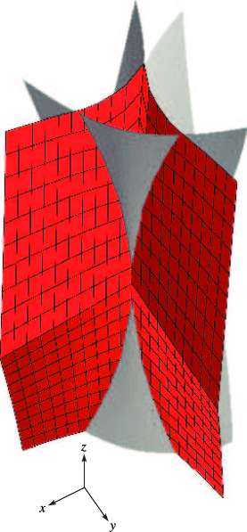
§36.5 Stokes Sets

►

§36.5(i) Definitions

… ►

§36.5(ii) Cuspoids

… ►

§36.5(iv) Visualizations

… ►

►►

Figure 36.5.9: Sheets of the Stokes surface for the hyperbolic umbilic catastrophe (colored and with mesh) and the bifurcation set (gray). Magnify

2: Bibliography W

… ►

The Stokes set of the cusp diffraction catastrophe. J. Phys. A 13 (9), pp. 2913–2928.

ⓘ

External Links:

ISSN 0305-4470, Document, MathReview (I. Stewart), ZentralBlatt

Referenced by:

§36.5(ii).

Encodings:

BibTeX

…

3: 2.7 Differential Equations

… ►To include the point at infinity in the foregoing classification scheme, we transform it into the origin by replacing $z$ in (2.7.1) with $1/z$; see Olver (1997b, pp. 153–154). … ►in which $C_1$, $C_2$ are constants, the so-called Stokes multipliers. … ►For the calculation of Stokes multipliers see Olde Daalhuis and Olver (1995b). … ►We cannot take $f=x$ and $g=\ln x$ because $\int g{f}^{-1/2}dx$ would diverge as $x\to +\mathrm{\infty }$. Instead set $f=x+\ln x$, $g=0$. …

4: 7.20 Mathematical Applications

… ►For applications of the complementary error function in uniform asymptotic approximations of integrals—saddle point coalescing with a pole or saddle point coalescing with an endpoint—see Wong (1989, Chapter 7), Olver (1997b, Chapter 9), and van der Waerden (1951). ►The complementary error function also plays a ubiquitous role in constructing exponentially-improved asymptotic expansions and providing a smooth interpretation of the Stokes phenomenon; see §§2.11(iii) and 2.11(iv). … ►Let the set $\{x(t),y(t),t\}$ be defined by $x(t)=C\left(t\right)$, $y(t)=S\left(t\right)$, $t\ge 0$. Then the set $\{x(t),y(t)\}$ is called Cornu’s spiral: it is the projection of the corkscrew on the $\{x,y\}$-plane. …Furthermore, because $dy/dx=\tan \left(\frac{1}{2}\pi t^2\right)$, the angle between the $x$-axis and the tangent to the spiral at $P(t)$ is given by $\frac{1}{2}\pi t^2$. …

5: 1.6 Vectors and Vector-Valued Functions

… ►Note: The terminology open and closed sets and boundary points in the $(x,y)$ plane that is used in this subsection and §1.6(v) is analogous to that introduced for the complex plane in §1.9(ii). … ►and $S$ be the closed and bounded point set in the $(x,y)$ plane having a simple closed curve $C$ as boundary. … ►with $(u,v)\in D$, an open set in the plane. … ►

Stokes’s Theorem

…

6: Bibliography S

… ►

Some properties of polynomial sets of type zero. Duke Math. J. 5, pp. 590–622.

ⓘ

External Links:

ISSN 0012-7094, Link, MathReview (A. Erdélyi), ZentralBlatt

Referenced by:

§18.2(xii).

Encodings:

BibTeX

… ►

Effective calculation of the incomplete gamma function for parameter values $\alpha =(2n+1)/2$, $n=0,\mathrm{\dots },5$ . Angew. Informatik 17, pp. 30–32.

ⓘ

Notes:

Includes Fortran code.

External Links:

ZentralBlatt

Referenced by:

§8.28(ii).

Encodings:

BibTeX

… ►

Computation of angular momentum coefficients using sets of generalized hypergeometric functions. Comput. Phys. Comm. 22 (2-3), pp. 297–302.

ⓘ

External Links:

Document

Referenced by:

§34.13.

Encodings:

BibTeX

… ►

A stable quotient-difference algorithm. Math. Comp. 34 (150), pp. 515–519.

ⓘ

External Links:

ISSN 0025-5718, FullText, MathReview, ZentralBlatt

Referenced by:

§3.10(ii).

Encodings:

BibTeX

… ►

On certain special sets of orthogonal polynomials. Proc. Amer. Math. Soc. 1, pp. 731–737.

ⓘ

External Links:

ISSN 0002-9939, Document, Link, MathReview (A. C. Offord)

Referenced by:

§18.35(i).

Encodings:

BibTeX

…

7: 7.12 Asymptotic Expansions

… ►For these and other error bounds see Olver (1997b, pp. 109–112), with $\alpha =\frac{1}{2}$ and $z$ replaced by $z^2$; compare (7.11.2). ►For re-expansions of the remainder terms leading to larger sectors of validity, exponential improvement, and a smooth interpretation of the Stokes phenomenon, see §§2.11(ii)–2.11(iv) and use (7.11.3). … ►

7.12.2 $$\mathrm{f}\left(z\right)\sim \frac{1}{\pi z}\sum _{m=0}^{\mathrm{\infty }}{(-1)}^m\frac{{\left(\frac{1}{2}\right)}_{2m}}{{(\pi z^2/2)}^{2m}},$$

ⓘ

Symbols:

$\mathrm{f}\left(z\right)$: auxiliary function for Fresnel integrals, ${\left(a\right)}_n$: Pochhammer’s symbol (or shifted factorial), $\sim$: Poincaré asymptotic expansion, $\pi$: the ratio of the circumference of a circle to its diameter and $z$: complex variable

A&S Ref:

7.3.27

Referenced by:

§7.12(ii), §7.12(ii), Erratum (V1.0.9) for Chapters 7, 25

Permalink:

http://dlmf.nist.gov/7.12.E2

Encodings:

pMML, png, TeX

Notational Change (effective with 1.0.9):

Previously the RHS of this equation was written as $\frac{1}{\pi z}{\sum }_{m=0}^{\mathrm{\infty }}{(-1)}^m\frac{1\cdot 3\cdot 5\mathrm{\cdots }(4m-1)}{{(\pi z^2)}^{2m}}$. We have rewritten the sum more concisely using Pochhammer’s symbol.

Suggested 2014-03-13 by Giorgos Karagounis

See also:

Annotations for §7.12(ii), §7.12 and Ch.7

… ►

7.12.6 $$R_n^{(\mathrm{f})}(z)=\frac{{(-1)}^n}{\pi \sqrt{2}}{\int }_0^{\mathrm{\infty }}\frac{{\mathrm{e}}^{-\pi z^{2}t/2}{t}^{2n-(1/2)}}{t^2+1}dt,$$

ⓘ

Defines:

$R_n^{(\mathrm{f})}(z)$: remainder term (locally)

Symbols:

$\pi$: the ratio of the circumference of a circle to its diameter, $dx$: differential of $x$ , $\mathrm{e}$: base of natural logarithm, $\int$: integral, $z$: complex variable and $n$: nonnegative integer

A&S Ref:

7.3.29 (in different form)

Referenced by:

§7.12(ii)

Permalink:

http://dlmf.nist.gov/7.12.E6

Encodings:

pMML, png, TeX

See also:

Annotations for §7.12(ii), §7.12 and Ch.7

►

7.12.7 $$R_n^{(\mathrm{g})}(z)=\frac{{(-1)}^n}{\pi \sqrt{2}}{\int }_0^{\mathrm{\infty }}\frac{{\mathrm{e}}^{-\pi z^{2}t/2}{t}^{2n+(1/2)}}{t^2+1}dt.$$

ⓘ

Defines:

$R_n^{(\mathrm{g})}(z)$: remainder term (locally)

Symbols:

$\pi$: the ratio of the circumference of a circle to its diameter, $dx$: differential of $x$ , $\mathrm{e}$: base of natural logarithm, $\int$: integral, $z$: complex variable and $n$: nonnegative integer

A&S Ref:

7.3.30 (in different form)

Referenced by:

§7.12(ii)

Permalink:

http://dlmf.nist.gov/7.12.E7

Encodings:

pMML, png, TeX

See also:

Annotations for §7.12(ii), §7.12 and Ch.7

…

8: 3.10 Continued Fractions

… ►can be converted into a continued fraction $C$ of type (3.10.1), and with the property that the $n$th convergent $C_n=A_n/B_n$ to $C$ is equal to the $n$th partial sum of the series in (3.10.3), that is, … ►A more stable version of the algorithm is discussed in Stokes (1980). … ►This forward algorithm achieves efficiency and stability in the computation of the convergents $C_n=A_n/B_n$, and is related to the forward series recurrence algorithm. … ►

$D_1=1/b_1,$

… ►The recurrences are continued until $(\nabla C_n)/C_n$ is within a prescribed relative precision. …

9: 2.11 Remainder Terms; Stokes Phenomenon

§2.11 Remainder Terms; Stokes Phenomenon

… ►

§2.11(iv) Stokes Phenomenon

… ►That the change in their forms is discontinuous, even though the function being approximated is analytic, is an example of the Stokes phenomenon. Where should the change-over take place? Can it be accomplished smoothly? … ►For higher-order Stokes phenomena see Olde Daalhuis (2004b) and Howls et al. (2004). …

10: 6.12 Asymptotic Expansions

… ►For re-expansions of the remainder term leading to larger sectors of validity, exponential improvement, and a smooth interpretation of the Stokes phenomenon, see §§2.11(ii)–2.11(iv), with $p=1$. …