Simpson%20rule

SearchAdvancedHelp

(0.002 seconds)

1—10 of 126 matching pages

1: 3.5 Quadrature

… ►

§3.5(ii) Simpson’s Rule

… ►Then the elementary Simpson’s rule is … ►Then the composite Simpson’s rule is … ► ►Rules of closed type include the Newton–Cotes formulas such as the trapezoidal rules and Simpson’s rule. …

2: 3.8 Nonlinear Equations

… ►

§3.8(ii) Newton’s Rule

… ► … ►Newton’s rule is given by … ►Another iterative method is Halley’s rule: …The rule converges locally and is cubically convergent. …

3: 18.40 Methods of Computation

… ►Results of low ($2$ to $3$ decimal digits) precision for $w(x)$ are easily obtained for $N\sim 10$ to $20$. … ►

Derivative Rule Approach

►An alternate, and highly efficient, approach follows from the derivative rule conjecture, see Yamani and Reinhardt (1975), and references therein, namely that … ►

►►

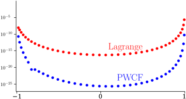
Figure 18.40.2: Derivative Rule inversions for $w^{\mathrm{RCP}}(x)$ carried out via Lagrange and PWCF interpolations. … Magnify

►Further, exponential convergence in $N$, via the Derivative Rule, rather than the power-law convergence of the histogram methods, is found for the inversion of Gegenbauer, Attractive, as well as Repulsive, Coulomb–Pollaczek, and Hermite weights and zeros to approximate $w(x)$ for these OP systems on $x\in [-1,1]$ and $(-\mathrm{\infty },\mathrm{\infty })$ respectively, Reinhardt (2018), and Reinhardt (2021b), Reinhardt (2021a). …

4: 20 Theta Functions

Chapter 20 Theta Functions

…

5: Bibliography R

… ►

On the definition and properties of generalized $6$-$j$ symbols. J. Math. Phys. 20 (12), pp. 2398–2415.

ⓘ

External Links:

ISSN 0022-2488, Document, MathReview (S. Saran), ZentralBlatt

Referenced by:

§16.4(iii), §16.4(iii).

Encodings:

BibTeX

… ►

Universality properties of Gaussian quadrature, the derivative rule, and a novel approach to Stieltjes inversion.

ⓘ

Notes:

arXiv:1812.02196

Referenced by:

§18.40(ii).

Encodings:

BibTeX

►

Erratum to:Relationships between the zeros, weights, and weight functions of orthogonal polynomials: Derivative rule approach to Stieltjes and spectral imaging. Computing in Science and Engineering 23 (4), pp. 91.

ⓘ

External Links:

ISSN 1521-9615, Document, Link

Referenced by:

§18.39(iv), §18.40(ii).

Encodings:

BibTeX

►

Relationships between the zeros, weights, and weight functions of orthogonal polynomials: Derivative rule approach to Stieltjes and spectral imaging. Computing in Science and Engineering 23 (3), pp. 56–64.

ⓘ

External Links:

ISSN 1521-9615, Document, Link

Referenced by:

§18.39(iv), §18.40(ii).

Encodings:

BibTeX

… ►

Finite-sum rules for Macdonald’s functions and Hankel’s symbols. Integral Transform. Spec. Funct. 10 (2), pp. 115–124.

ⓘ

External Links:

ISSN 1065-2469, Document, MathReview, ZentralBlatt

Referenced by:

§10.60(iii).

Encodings:

BibTeX

…

6: Bibliography

… ►

Exact linearization of a Painlevé transcendent. Phys. Rev. Lett. 38 (20), pp. 1103–1106.

ⓘ

External Links:

Document, MathReview (Mark Adler)

Referenced by:

§32.11(ii), §32.13(i), §32.13(ii), §32.13(iii), §32.5.

Encodings:

BibTeX

… ►

Numerical computation of Tricomi’s psi function by the trapezoidal rule. Computing 39 (3), pp. 271–279.

ⓘ

External Links:

ISSN 0010-485X, Document, MathReview, ZentralBlatt

Referenced by:

§13.29(iii).

Encodings:

BibTeX

►

Numerical evaluation of the Kummer function with complex argument by the trapezoidal rule. Rend. Sem. Mat. Univ. Politec. Torino 49 (3), pp. 315–327.

ⓘ

External Links:

ISSN 0373-1243, MathReview, ZentralBlatt

Referenced by:

§13.29(iii).

Encodings:

BibTeX

►

Numerical calculation of incomplete gamma functions by the trapezoidal rule. Numer. Math. 50 (4), pp. 419–428.

ⓘ

External Links:

ISSN 0029-599X, Document, MathReview (F. W. J. Olver), ZentralBlatt

Referenced by:

§8.25(ii).

Encodings:

BibTeX

►

Numerical Calculation of the Riemann Zeta Function and Generalizations by Means of the Trapezoidal Rule. In Numerical and Applied Mathematics, Part II (Paris, 1988), C. Brezinski (Ed.), IMACS Ann. Comput. Appl. Math., Vol. 1, pp. 467–472.

ⓘ

External Links:

MathReview

Referenced by:

§25.18(i).

Encodings:

BibTeX

…

7: Bibliography G

… ►

Stable computation of high order Gauss quadrature rules using discretization for measures in radiation transfer. J. Quant. Spectrosc. Radiat. Transfer 68 (2), pp. 213–223.

ⓘ

Referenced by:

§18.39(iii).

Encodings:

BibTeX

… ►

Algorithm 726: ORTHPOL — a package of routines for generating orthogonal polynomials and Gauss-type quadrature rules. ACM Trans. Math. Software 20 (1), pp. 21–62.

ⓘ

Notes:

For remark see same journal 24(1998), p. 355.

External Links:

Document, ISSN 0098-3500, GAMS (module 726; package TOMS), ZentralBlatt

Referenced by:

2nd item, §3.5(v), §3.5(v).

Encodings:

BibTeX

… ►

Computing special functions by using quadrature rules. Numer. Algorithms 33 (1-4), pp. 265–275.

ⓘ

Notes:

International Conference on Numerical Algorithms, Vol. I (Marrakesh, 2001)

External Links:

ISSN 1017-1398, Document, MathReview, ZentralBlatt

Referenced by:

§3.5(ix).

Encodings:

BibTeX

… ►

Algorithm 939: computation of the Marcum Q-function. ACM Trans. Math. Softw. 40 (3), pp. 20:1–20:21.

ⓘ

Notes:

Includes Fortran program claiming 12S accuracy

External Links:

ISSN 0098-3500, Link, Document, MathReview Entry, ZentralBlatt

Referenced by:

3rd item, §10.77(ix).

Encodings:

BibTeX

… ►

Calculation of Gauss quadrature rules. Math. Comp. 23 (106), pp. 221–230.

ⓘ

Notes:

Loose microfiche suppl. A1–A10

External Links:

FullText, MathReview (F. Stenger), ZentralBlatt

Referenced by:

§18.39(iii), §3.5(vi).

Encodings:

BibTeX

…

8: 1.11 Zeros of Polynomials

… ►

Descartes’ Rule of Signs

… ►Resolvent cubic is $z^3+12z^2+20z+9=0$ with roots ${\theta }_1=-1$, ${\theta }_2=-\frac{1}{2}(11+\sqrt{85})$, ${\theta }_3=-\frac{1}{2}(11-\sqrt{85})$, and $\sqrt{-{\theta }_1}=1$, $\sqrt{-{\theta }_2}=\frac{1}{2}(\sqrt{17}+\sqrt{5})$, $\sqrt{-{\theta }_3}=\frac{1}{2}(\sqrt{17}-\sqrt{5})$. …

9: 3.4 Differentiation

… ►

$$B_{-2}^5=\frac{1}{120}(6-10t-15t^2+20t^3-5t^4),$$

… ►

$$B_{-3}^6=-\frac{1}{720}(12-8t-45t^2+20t^3+15t^4-6t^5),$$

►

$$B_{-2}^6=\frac{1}{60}(9-9t-30t^2+20t^3+5t^4-3t^5),$$

… ►The integral on the right-hand side can be approximated by the composite trapezoidal rule (3.5.2). … ►As explained in §§3.5(i) and 3.5(ix) the composite trapezoidal rule can be very efficient for computing integrals with analytic periodic integrands. …

10: 8 Incomplete Gamma and Related
Functions

…