SL(2,Z) bilinear transformation
(0.004 seconds)
21—30 of 814 matching pages
21: Bibliography E
…
►
The numerical inversion of two classes of Kontorovich-Lebedev transform by direct quadrature.
J. Comput. Appl. Math. 61 (1), pp. 43–72.
…
►
Tables of Integral Transforms. Vol. I.
McGraw-Hill Book Company, Inc., New York-Toronto-London.
►
Tables of Integral Transforms. Vol. II.
McGraw-Hill Book Company, Inc., New York-Toronto-London.
…
►
Painlevé transcendent describes quantum correlation function of the antiferromagnet away from the free-fermion point.
J. Phys. A 29 (17), pp. 5619–5626.
…
►
On the transformation theory of ordinary second-order linear symmetric differential expressions.
Czechoslovak Math. J. 32(107) (2), pp. 275–306.
…
22: 2.4 Contour Integrals
…
►For examples and extensions (including uniformity and loop integrals) see Olver (1997b, Chapter 4), Wong (1989, Chapter 1), and Temme (1985).
►
(b)
…
§2.4(ii) Inverse Laplace Transforms
… ►Then the Laplace transform … ►For examples see Olver (1997b, pp. 315–320). … ►ranges along a ray or over an annular sector , , where , , and . converges at absolutely and uniformly with respect to .
23: 15.14 Integrals
§15.14 Integrals
►The Mellin transform of the hypergeometric function of negative argument is given by … ►Fourier transforms of hypergeometric functions are given in Erdélyi et al. (1954a, §§1.14 and 2.14). Laplace transforms of hypergeometric functions are given in Erdélyi et al. (1954a, §4.21), Oberhettinger and Badii (1973, §1.19), and Prudnikov et al. (1992a, §3.37). …Hankel transforms of hypergeometric functions are given in Oberhettinger (1972, §1.17) and Erdélyi et al. (1954b, §8.17). …24: Bibliography P
…
►
A Kummer-type transformation for a hypergeometric function.
J. Comput. Appl. Math. 173 (2), pp. 379–382.
…
►
Complex zeros of the modified Bessel function
.
Math. Comp. 26 (120), pp. 949–953.
…
►
Bounds for ratios of modified Bessel functions.
Integral Transform. Spec. Funct. 9 (4), pp. 293–298.
…
►
Fourier Series and Integral Transforms.
Cambridge University Press, Cambridge.
…
►
Integrals and Series: Direct Laplace Transforms, Vol. 4.
Gordon and Breach Science Publishers, New York.
…
25: 35.8 Generalized Hypergeometric Functions of Matrix Argument
26: 2.5 Mellin Transform Methods
…
►
…
►In the half-plane , the product has a pole of order two at each positive integer, and
…
►By Table 2.5.1, is an analytic function in the half-plane .
…
►Alternatively, if in (2.5.18), then can be continued analytically to an entire function.
►Since is analytic for by Table 2.5.1, the analytically-continued allows us to extend the Mellin transform of via
…
27: 22.7 Landen Transformations
§22.7 Landen Transformations
►§22.7(i) Descending Landen Transformation
… ►§22.7(ii) Ascending Landen Transformation
… ►§22.7(iii) Generalized Landen Transformations
…28: 22.16 Related Functions
…
►With as in (22.2.1) and ,
…
►In Equations (22.16.24)–(22.16.26), .
…
►where .
…
►(Sometimes in the literature is denoted by .)
…
►
satisfies the same quasi-addition formula as the function , given by (22.16.27).
…
29: 35.7 Gaussian Hypergeometric Function of Matrix Argument
…
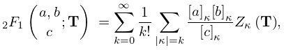
►
35.7.1
, ;
.
…
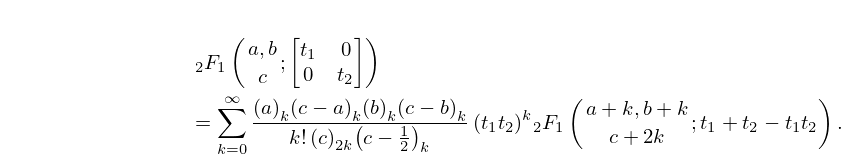
►
Case
►
35.7.3
…
►
Transformations of Parameters
… ►Subject to the conditions (a)–(c), the function is the unique solution of each partial differential equation …30: 19.15 Advantages of Symmetry
…
►The function (Carlson (1963)) reveals the full permutation symmetry that is partially hidden in , and leads to symmetric standard integrals that simplify many aspects of theory, applications, and numerical computation.
►Symmetry in of , , and replaces the five transformations (19.7.2), (19.7.4)–(19.7.7) of Legendre’s integrals; compare (19.25.17).
Symmetry unifies the Landen transformations of §19.8(ii) with the Gauss transformations of §19.8(iii), as indicated following (19.22.22) and (19.36.9).
(19.21.12) unifies the three transformations in §19.7(iii) that change the parameter of Legendre’s third integral.
…
