SL(2,Z) bilinear transformation

SearchAdvancedHelp

(0.004 seconds)

11—20 of 814 matching pages

11: 10.43 Integrals

… ►Let ${𝒵}_{\nu }\left(z\right)$ be defined as in §10.25(ii). … ►

§10.43(v) Kontorovich–Lebedev Transform

►The Kontorovich–Lebedev transform of a function $g(x)$ is defined as … ►For asymptotic expansions of the direct transform (10.43.30) see Wong (1981), and for asymptotic expansions of the inverse transform (10.43.31) see Naylor (1990, 1996). ►For collections of the Kontorovich–Lebedev transform, see Erdélyi et al. (1954b, Chapter 12), Prudnikov et al. (1986b, pp. 404–412), and Oberhettinger (1972, Chapter 5). …

12: 25.3 Graphics

… ►

►►

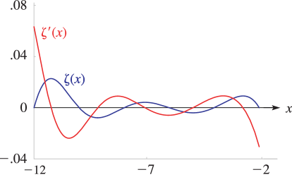
Figure 25.3.2: Riemann zeta function $\zeta \left(x\right)$ and its derivative ${\zeta }^{\prime }\left(x\right)$, $-12\le x\le -2$. Magnify

… ►

►►

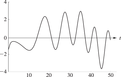
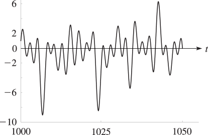
Figure 25.3.4: $Z(t)$, $0\le t\le 50$. $Z(t)$ and $\zeta \left(\frac{1}{2}+\mathrm{i}t\right)$ have the same zeros. … Magnify

►

►►

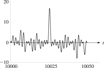
Figure 25.3.5: $Z(t)$, $1000\le t\le 1050$. Magnify

►

►►

Figure 25.3.6: $Z(t)$, $10000\le t\le 10050$. Magnify

13: 1.9 Calculus of a Complex Variable

… ► ►

Bilinear Transformation

… ►The cross ratio of $z_1,z_2,z_3,z_4\in ℂ\cup \{\mathrm{\infty }\}$ is defined by …or its limiting form, and is invariant under bilinear transformations. ►Other names for the bilinear transformation are fractional linear transformation, homographic transformation, and Möbius transformation. …

14: 19.36 Methods of Computation

… ►

§19.36(ii) Quadratic Transformations

… ►Descending Gauss transformations of $\mathrm{\Pi }(\varphi ,{\alpha }^2,k)$ (see (19.8.20)) are used in Fettis (1965) to compute a large table (see §19.37(iii)). …If ${\alpha }^2=k^2$, then the method fails, but the function can be expressed by (19.6.13) in terms of $E(\varphi ,k)$, for which Neuman (1969b) uses ascending Landen transformations. … ►Quadratic transformations can be applied to compute Bulirsch’s integrals (§19.2(iii)). …The function $\mathrm{el2}(x,k_c,a,b)$ is computed by descending Landen transformations if $x$ is real, or by descending Gauss transformations if $x$ is complex (Bulirsch (1965b)). …

15: 25.10 Zeros

… ►Calculations relating to the zeros on the critical line make use of the real-valued function …is chosen to make $Z(t)$ real, and $\mathrm{ph}\mathrm{\Gamma }\left(\frac{1}{4}+\frac{1}{2}\mathrm{i}t\right)$ assumes its principal value. Because $|Z(t)|=|\zeta \left(\frac{1}{2}+\mathrm{i}t\right)|$, $Z(t)$ vanishes at the zeros of $\zeta \left(\frac{1}{2}+\mathrm{i}t\right)$, which can be separated by observing sign changes of $Z(t)$. Because $Z(t)$ changes sign infinitely often, $\zeta \left(\frac{1}{2}+\mathrm{i}t\right)$ has infinitely many zeros with $t$ real. … ►Sign changes of $Z(t)$ are determined by multiplying (25.9.3) by $\exp \left(\mathrm{i}\vartheta (t)\right)$ to obtain the Riemann–Siegel formula: …

16: 35.4 Partitions and Zonal Polynomials

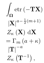
… ►For any partition $\kappa$, the zonal polynomial $Z_{\kappa }:𝓢\to ℝ$ is defined by the properties … ►Therefore $Z_{\kappa }\left(𝐓\right)$ is a symmetric polynomial in the eigenvalues of $𝐓$. … ►For $k=0,1,2,\mathrm{\dots }$, … ►For $𝐓\in 𝛀$ and $\mathrm{\Re }\left(a\right),\mathrm{\Re }\left(b\right)>\frac{1}{2}(m-1)$, ►

35.4.8 $${\int }_{𝛀}\mathrm{etr}\left(-𝐓𝐗\right){\left|𝐗\right|}^{a-\frac{1}{2}(m+1)}{Z}_{\kappa }\left(𝐗\right)d𝐗={\mathrm{\Gamma }}_m\left(a+\kappa \right){\left|𝐓\right|}^{-a}{Z}_{\kappa }\left({𝐓}^{-1}\right),$$

ⓘ

Symbols:

$\mathrm{etr}\left(𝐀\right)$: exponential of trace, $\int$: integral, ${\mathrm{\Gamma }}_m\left(a\right)$: multivariate gamma function, $Z_{\kappa }\left(𝐓\right)$: zonal polynomial, $a$: complex variable, $𝐓$: real symmetric $m\times m$ matrix, $𝐗$: real symmetric $m\times m$ matrix, $\left|𝐗\right|$: determinant of $𝐗$ , $d$: differential of matrix, $𝛀$: space of positive-definite real symmetric $m\times m$ matrices, $m$: positive integer and $\kappa$: vector of nonnegative integers

Permalink:

http://dlmf.nist.gov/35.4.E8

Encodings:

pMML, png, TeX

See also:

Annotations for §35.4(ii), §35.4(ii), §35.4 and Ch.35

…

17: 10.44 Sums

… ►

10.44.1 $${𝒵}_{\nu }\left(\lambda z\right)={\lambda }^{\pm \nu }\sum _{k=0}^{\mathrm{\infty }}\frac{{({\lambda }^2-1)}^k{(\frac{1}{2}z)}^k}{k!}{𝒵}_{\nu \pm k}\left(z\right),$$ .

ⓘ

Symbols:

$!$: factorial (as in $n!$), ${𝒵}_{\nu }\left(z\right)$: modified cylinder function, $k$: nonnegative integer, $z$: complex variable and $\nu$: complex parameter

A&S Ref:

9.6.51

Referenced by:

§10.44(i), §10.66

Permalink:

http://dlmf.nist.gov/10.44.E1

Encodings:

pMML, png, TeX

See also:

Annotations for §10.44(i), §10.44 and Ch.10

►If $𝒵=I$ and the upper signs are taken, then the restriction on $\lambda$ is unnecessary. … ►

10.44.3 $${𝒵}_{\nu }\left(u\pm v\right)=\sum _{k=-\mathrm{\infty }}^{\mathrm{\infty }}{(\pm 1)}^k{𝒵}_{\nu +k}\left(u\right)I_k\left(v\right),$$ .

ⓘ

Symbols:

$I_{\nu }\left(z\right)$: modified Bessel function of the first kind, ${𝒵}_{\nu }\left(z\right)$: modified cylinder function, $k$: nonnegative integer and $\nu$: complex parameter

Permalink:

http://dlmf.nist.gov/10.44.E3

Encodings:

pMML, png, TeX

See also:

Annotations for §10.44(ii), §10.44(ii), §10.44 and Ch.10

►The restriction is unnecessary when $𝒵=I$ and $\nu$ is an integer. … ►

10.44.6 $$K_n\left(z\right)=\frac{n!{(\frac{1}{2}z)}^{-n}}{2}\sum _{k=0}^{n-1}{(-1)}^k\frac{{(\frac{1}{2}z)}^k{I}_k\left(z\right)}{k!(n-k)}+{(-1)}^{n-1}\left(\ln \left(\frac{1}{2}z\right)-\psi \left(n+1\right)\right)I_n\left(z\right)+{(-1)}^n\sum _{k=1}^{\mathrm{\infty }}\frac{(n+2k)I_{n+2k}\left(z\right)}{k(n+k)},$$

ⓘ

Symbols:

$\psi \left(z\right)$: psi (or digamma) function, $!$: factorial (as in $n!$), $I_{\nu }\left(z\right)$: modified Bessel function of the first kind, $K_{\nu }\left(z\right)$: modified Bessel function of the second kind, $\ln z$: principal branch of logarithm function, $n$: integer, $k$: nonnegative integer and $z$: complex variable

A&S Ref:

9.6.53

Permalink:

http://dlmf.nist.gov/10.44.E6

Encodings:

pMML, png, TeX

See also:

Annotations for §10.44(iii), §10.44 and Ch.10

…

18: 19.19 Taylor and Related Series

… ►For $N=0,1,2,\mathrm{\dots }$ define the homogeneous hypergeometric polynomial … ►If $n=2$, then (19.19.3) is a Gauss hypergeometric series (see (19.25.43) and (15.2.1)). … ►and define the $n$-tuple $\frac{\mathrm{𝟏}}{\mathrm{𝟐}}=(\frac{1}{2},\mathrm{\dots },\frac{1}{2})$. … ►The number of terms in $T_N$ can be greatly reduced by using variables $𝐙=\mathrm{𝟏}-(𝐳/A)$ with $A$ chosen to make $E_1(𝐙)=0$. … ►

19.19.7 $$R_{-a}(\frac{\mathrm{𝟏}}{\mathrm{𝟐}};𝐳)=A^{-a}\sum _{N=0}^{\mathrm{\infty }}\frac{{\left(a\right)}_N}{{\left(\frac{1}{2}n\right)}_N}{T}_N(\frac{\mathrm{𝟏}}{\mathrm{𝟐}},𝐙),$$

ⓘ

Symbols:

$R_{-a}(b_1,\mathrm{\dots },b_n;z_1,\mathrm{\dots },z_n)$ or $R_{-a}(𝐛;𝐳)$: multivariate hypergeometric function, ${\left(a\right)}_n$: Pochhammer’s symbol (or shifted factorial), $n$: nonnegative integer, $N$: nonnegative integer, $T_N(𝐛,𝐳)$: polynomial, $𝐙$: variable and $A$

Referenced by:

§19.15, §19.36(i), §19.36(i), §19.36(i)

Permalink:

http://dlmf.nist.gov/19.19.E7

Encodings:

pMML, png, TeX

See also:

Annotations for §19.19 and Ch.19

…

19: 18.38 Mathematical Applications

… ►It has elegant structures, including $N$-soliton solutions, Lax pairs, and Bäcklund transformations. While the Toda equation is an important model of nonlinear systems, the special functions of mathematical physics are usually regarded as solutions to linear equations. However, by using Hirota’s technique of bilinear formalism of soliton theory, Nakamura (1996) shows that a wide class of exact solutions of the Toda equation can be expressed in terms of various special functions, and in particular classical OP’s. … ►

Radon Transform

… ►Define a further operator $K_2$ by …

20: Bibliography

… ►

Solitons and the Inverse Scattering Transform. SIAM Studies in Applied Mathematics, Vol. 4, Society for Industrial and Applied Mathematics (SIAM), Philadelphia, PA.

ⓘ

External Links:

ISBN 0-89871-174-6, MathReview (Benno Fuchssteiner), ZentralBlatt

Referenced by:

§21.9, §21.9, §32.5, §9.16, Profile Mark J. Ablowitz.

Encodings:

BibTeX

… ►

Lectures on Integral Transforms. Translations of Mathematical Monographs, Vol. 70, American Mathematical Society, Providence, RI.

ⓘ

Notes:

Translated from the Russian by H. H. McFaden

External Links:

ISBN 0-8218-4524-1, MathReview, ZentralBlatt

Referenced by:

§10.22(v).

Encodings:

BibTeX

… ►

Transformations $R{S}_4^2(3)$ of the ranks $\le 4$ and algebraic solutions of the sixth Painlevé equation. Comm. Math. Phys. 228 (1), pp. 151–176.

ⓘ

External Links:

ISSN 0010-3616, Document, MathReview (Andrei A. Kapaev), ZentralBlatt

Referenced by:

§32.9(iii).

Encodings:

BibTeX

… ►

Summations and transformations for basic Appell series. J. London Math. Soc. (2) 4, pp. 618–622.

ⓘ

External Links:

MathReview (R. N. Jain), ZentralBlatt

Referenced by:

§17.11.

Encodings:

BibTeX

… ►

Jacobi polynomials. I. New proofs of Koornwinder’s Laplace type integral representation and Bateman’s bilinear sum. SIAM J. Math. Anal. 5, pp. 119–124.

ⓘ

External Links:

ISSN 1095-7154, Document, MathReview (R. P. Soni), ZentralBlatt

Referenced by:

§18.18(iv).

Encodings:

BibTeX

…