SL(2,Z)

SearchAdvancedHelp

(0.002 seconds)

1—10 of 803 matching pages

1: 23.15 Definitions

… ►

$k={\displaystyle \frac{{\theta }_2^2(0,q)}{{\theta }_3^2(0,q)}},$

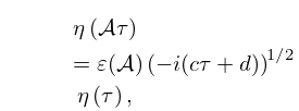
… ►The set of all bilinear transformations of this form is denoted by SL $(2,\mathbb{Z})$ (Serre (1973, p. 77)). ►A modular function $f(\tau )$ is a function of $\tau$ that is meromorphic in the half-plane $\mathrm{\Im }\tau >0$, and has the property that for all $𝒜\in \text{<span class="ltx\_text hilite">SL</span>}(2,\mathbb{Z})$, or for all $𝒜$ belonging to a subgroup of SL $(2,\mathbb{Z})$, …(Some references refer to $2\mathrm{\ell }$ as the level). …

2: 10.29 Recurrence Relations and Derivatives

… ►With ${𝒵}_{\nu }\left(z\right)$ defined as in §10.25(ii), ►

${𝒵}_{\nu -1}\left(z\right)-{𝒵}_{\nu +1}\left(z\right)=(2\nu /z){𝒵}_{\nu }\left(z\right),$

►

${𝒵}_{\nu -1}\left(z\right)+{𝒵}_{\nu +1}\left(z\right)=2{𝒵}_{\nu }^{\prime }\left(z\right).$

… ►For results on modified quotients of the form $z{𝒵}_{\nu \pm 1}\left(z\right)/{𝒵}_{\nu }\left(z\right)$ see Onoe (1955) and Onoe (1956). … ►For $k=0,1,2,\mathrm{\dots }$, …

3: 15.17 Mathematical Applications

… ►First, as spherical functions on noncompact Riemannian symmetric spaces of rank one, but also as associated spherical functions, intertwining functions, matrix elements of SL $(2,ℝ)$, and spherical functions on certain nonsymmetric Gelfand pairs. …

4: 23.18 Modular Transformations

… ►and $\lambda \left(\tau \right)$ is a cusp form of level zero for the corresponding subgroup of SL $(2,\mathbb{Z})$. … ► $J\left(\tau \right)$ is a modular form of level zero for SL $(2,\mathbb{Z})$. … ►

23.18.5 $$\eta \left(𝒜\tau \right)=\epsilon (𝒜){\left(-\mathrm{i}(c\tau +d)\right)}^{1/2}\eta \left(\tau \right),$$

ⓘ

Symbols:

$\eta \left(\tau \right)$: Dedekind’s eta function (or Dedekind modular function), $\mathrm{i}$: imaginary unit, $\tau$: complex variable, $𝒜$: bilinear transformation, $c$: integer, $d$: integer and $\epsilon (𝒜)$: function

Permalink:

http://dlmf.nist.gov/23.18.E5

Encodings:

pMML, png, TeX

See also:

Annotations for §23.18, §23.18 and Ch.23

… ►

23.18.7 $$s(d,c)=\sum _{r=1}^{c-1}\frac{r}{c}\left(\frac{dr}{c}-\lfloor \frac{dr}{c}\rfloor -\frac{1}{2}\right),$$ $c>0$.

ⓘ

Symbols:

$\lfloor x\rfloor$: floor of $x$ , $\left(m,n\right)$: greatest common divisor (gcd), $c$: integer and $d$: integer

Referenced by:

§23.18, Erratum (V1.0.11) for Equation (23.18.7)

Permalink:

http://dlmf.nist.gov/23.18.E7

Encodings:

pMML, png, TeX

Errata (effective with 1.0.11):

Originally the sum ${\sum }_{r=1}^{c-1}$ was written with an additional constraint on the summation, that $\left(r,c\right)=1$. This additional condition was incorrect and has been removed.

Reported 2015-10-05 by Howard Cohl and Tanay Wakhare

See also:

Annotations for §23.18, §23.18 and Ch.23

… ►Note that $\eta \left(\tau \right)$ is of level $\frac{1}{2}$. …

5: 10.36 Other Differential Equations

… ►The quantity ${\lambda }^2$ in (10.13.1)–(10.13.6) and (10.13.8) can be replaced by $-{\lambda }^2$ if at the same time the symbol $𝒞$ in the given solutions is replaced by $𝒵$. … ►

10.36.1 $$z^2(z^2+{\nu }^2)w^{\prime \prime }+z(z^2+3{\nu }^2)w^{\prime }-\left({(z^2+{\nu }^2)}^2+z^2-{\nu }^2\right)w=0,$$ $w={𝒵}_{\nu }^{\prime }\left(z\right)$,

ⓘ

Symbols:

${𝒵}_{\nu }\left(z\right)$: modified cylinder function, $z$: complex variable and $\nu$: complex parameter

Permalink:

http://dlmf.nist.gov/10.36.E1

Encodings:

pMML, png, TeX

See also:

Annotations for §10.36 and Ch.10

►

10.36.2 $$z^2{w}^{\prime \prime }+z(1\pm 2z)w^{\prime }+(\pm z-{\nu }^2)w=0,$$ $w={\mathrm{e}}^{\mp z}{𝒵}_{\nu }\left(z\right)$.

ⓘ

Symbols:

$\mathrm{e}$: base of natural logarithm, ${𝒵}_{\nu }\left(z\right)$: modified cylinder function, $z$: complex variable and $\nu$: complex parameter

A&S Ref:

9.6.41

Permalink:

http://dlmf.nist.gov/10.36.E2

Encodings:

pMML, png, TeX

See also:

Annotations for §10.36 and Ch.10

…

6: 33.22 Particle Scattering and Atomic and Molecular Spectra

… ►With $\mathrm{e}$ denoting here the elementary charge, the Coulomb potential between two point particles with charges $Z_1\mathrm{e},Z_2\mathrm{e}$ and masses $m_1,m_2$ separated by a distance $s$ is $V(s)=Z_1{Z}_2{\mathrm{e}}^2/(4\pi {\epsilon }_{0}s)=Z_1{Z}_2\alpha \mathrm{\hslash }c/s$, where $Z_j$ are atomic numbers, ${\epsilon }_0$ is the electric constant, $\alpha$ is the fine structure constant, and $\mathrm{\hslash }$ is the reduced Planck’s constant. … ►In these applications, the $Z$-scaled variables $r$ and $ϵ$ are more convenient. ►

$Z$ Scaling

►The $Z$-scaled variables $r$ and $ϵ$ of §33.14 are given by … ►For $Z_1{Z}_2=-1$ and $m=m_{\mathrm{e}}$, the electron mass, the scaling factors in (33.22.5) reduce to the Bohr radius, $a_0=\mathrm{\hslash }/(m_{\mathrm{e}}c\alpha )$, and to a multiple of the Rydberg constant, …

7: 25.3 Graphics

… ►

►►

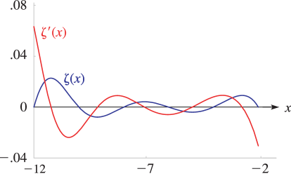
Figure 25.3.2: Riemann zeta function $\zeta \left(x\right)$ and its derivative ${\zeta }^{\prime }\left(x\right)$, $-12\le x\le -2$. Magnify

… ►

►►

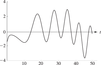
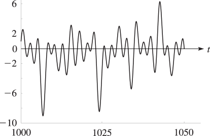
Figure 25.3.4: $Z(t)$, $0\le t\le 50$. $Z(t)$ and $\zeta \left(\frac{1}{2}+\mathrm{i}t\right)$ have the same zeros. … Magnify

►

►►

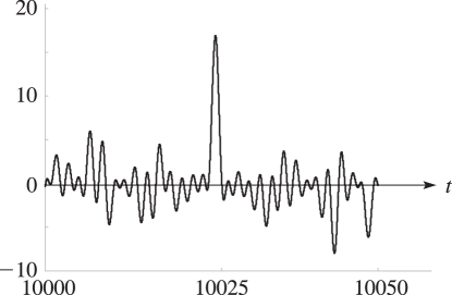
Figure 25.3.5: $Z(t)$, $1000\le t\le 1050$. Magnify

►

►►

Figure 25.3.6: $Z(t)$, $10000\le t\le 10050$. Magnify

8: 35.2 Laplace Transform

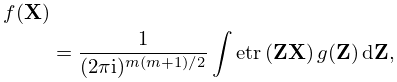
… ►For any complex symmetric matrix $𝐙$, … ►Then (35.2.1) converges absolutely on the region $\mathrm{\Re }\left(𝐙\right)>{𝐗}_0$, and $g(𝐙)$ is a complex analytic function of all elements $z_{j,k}$ of $𝐙$. … ►

35.2.2 $$f(𝐗)=\frac{1}{{(2\pi \mathrm{i})}^{m(m+1)/2}}\int \mathrm{etr}\left(𝐙𝐗\right)g(𝐙)d𝐙,$$

ⓘ

Symbols:

$\pi$: the ratio of the circumference of a circle to its diameter, $\mathrm{etr}\left(𝐀\right)$: exponential of trace, $\mathrm{i}$: imaginary unit, $\int$: integral, $𝐗$: real symmetric $m\times m$ matrix, $d$: differential of matrix, $𝐙$: complex symmetric $m\times m$ matrix, $f(𝐗)$: complex-valued function of matrix argument, $m$: positive integer and $g$: Laplace transformation of $f$

Permalink:

http://dlmf.nist.gov/35.2.E2

Encodings:

pMML, png, TeX

See also:

Annotations for §35.2, §35.2 and Ch.35

►where the integral is taken over all $𝐙=𝐔+\mathrm{i}𝐕$ such that $𝐔>{𝐗}_0$ and $𝐕$ ranges over $𝓢$. … ►If $g_j$ is the Laplace transform of $f_j$, $j=1,2$, then $g_1{g}_2$ is the Laplace transform of the convolution $f_1\ast f_2$, where …

9: 25.10 Zeros

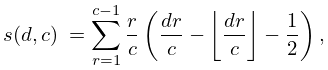
… ►Calculations relating to the zeros on the critical line make use of the real-valued function …is chosen to make $Z(t)$ real, and $\mathrm{ph}\mathrm{\Gamma }\left(\frac{1}{4}+\frac{1}{2}\mathrm{i}t\right)$ assumes its principal value. Because $|Z(t)|=|\zeta \left(\frac{1}{2}+\mathrm{i}t\right)|$, $Z(t)$ vanishes at the zeros of $\zeta \left(\frac{1}{2}+\mathrm{i}t\right)$, which can be separated by observing sign changes of $Z(t)$. Because $Z(t)$ changes sign infinitely often, $\zeta \left(\frac{1}{2}+\mathrm{i}t\right)$ has infinitely many zeros with $t$ real. … ►Sign changes of $Z(t)$ are determined by multiplying (25.9.3) by $\exp \left(\mathrm{i}\vartheta (t)\right)$ to obtain the Riemann–Siegel formula: …

10: 35.4 Partitions and Zonal Polynomials

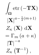
… ►For any partition $\kappa$, the zonal polynomial $Z_{\kappa }:𝓢\to ℝ$ is defined by the properties … ►Therefore $Z_{\kappa }\left(𝐓\right)$ is a symmetric polynomial in the eigenvalues of $𝐓$. … ►For $k=0,1,2,\mathrm{\dots }$, … ►For $𝐓\in 𝛀$ and $\mathrm{\Re }\left(a\right),\mathrm{\Re }\left(b\right)>\frac{1}{2}(m-1)$, ►

35.4.8 $${\int }_{𝛀}\mathrm{etr}\left(-𝐓𝐗\right){\left|𝐗\right|}^{a-\frac{1}{2}(m+1)}{Z}_{\kappa }\left(𝐗\right)d𝐗={\mathrm{\Gamma }}_m\left(a+\kappa \right){\left|𝐓\right|}^{-a}{Z}_{\kappa }\left({𝐓}^{-1}\right),$$

ⓘ

Symbols:

$\mathrm{etr}\left(𝐀\right)$: exponential of trace, $\int$: integral, ${\mathrm{\Gamma }}_m\left(a\right)$: multivariate gamma function, $Z_{\kappa }\left(𝐓\right)$: zonal polynomial, $a$: complex variable, $𝐓$: real symmetric $m\times m$ matrix, $𝐗$: real symmetric $m\times m$ matrix, $\left|𝐗\right|$: determinant of $𝐗$ , $d$: differential of matrix, $𝛀$: space of positive-definite real symmetric $m\times m$ matrices, $m$: positive integer and $\kappa$: vector of nonnegative integers

Permalink:

http://dlmf.nist.gov/35.4.E8

Encodings:

pMML, png, TeX

See also:

Annotations for §35.4(ii), §35.4(ii), §35.4 and Ch.35

…