Rydberg constant

SearchAdvancedHelp

(0.001 seconds)

1—10 of 435 matching pages

1: 33.22 Particle Scattering and Atomic and Molecular Spectra

… ►

§33.22(i) Schrödinger Equation

►With $\mathrm{e}$ denoting here the elementary charge, the Coulomb potential between two point particles with charges $Z_1\mathrm{e},Z_2\mathrm{e}$ and masses $m_1,m_2$ separated by a distance $s$ is $V(s)=Z_1{Z}_2{\mathrm{e}}^2/(4\pi {\epsilon }_{0}s)=Z_1{Z}_2\alpha \mathrm{\hslash }c/s$, where $Z_j$ are atomic numbers, ${\epsilon }_0$ is the electric constant, $\alpha$ is the fine structure constant, and $\mathrm{\hslash }$ is the reduced Planck’s constant. The reduced mass is $m=m_1{m}_2/(m_1+m_2)$, and at energy of relative motion $E$ with relative orbital angular momentum $\mathrm{\ell }\mathrm{\hslash }$, the Schrödinger equation for the radial wave function $w(s)$ is given by … ►For $Z_1{Z}_2=-1$ and $m=m_{\mathrm{e}}$, the electron mass, the scaling factors in (33.22.5) reduce to the Bohr radius, $a_0=\mathrm{\hslash }/(m_{\mathrm{e}}c\alpha )$, and to a multiple of the Rydberg constant, ► $R_{\mathrm{\infty }}=m_{\mathrm{e}}c{\alpha }^2/(2\mathrm{\hslash })$. …

2: Bibliography H

… ►

The combination of $R$-matrix and complex coordinate methods: Application to the diamagnetic Rydberg spectra of Ba and Sr. J. Phys. B 26 (12), pp. 1775–1790.

ⓘ

External Links:

ISSN 0953-4075, Document, MathReview

Referenced by:

4th item.

Encodings:

BibTeX

►

Formulae for growth factors in expanding universes containing matter and a cosmological constant. Monthly Notices Roy. Astronom. Soc. 322 (2), pp. 419–425.

ⓘ

External Links:

Document

Referenced by:

§8.24(ii).

Encodings:

BibTeX

… ►

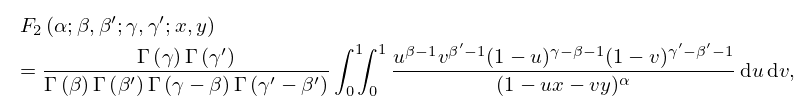
Note on Dr. Vacca’s series for $\gamma$ . Quart. J. Math. 43, pp. 215–216.

ⓘ

External Links:

ZentralBlatt

Referenced by:

(25.2.4), (25.2.5), §25.2(ii).

Encodings:

BibTeX

…

3: Bibliography

… ►

Tables of $\ln \mathrm{\Gamma }(z)$ for Complex Argument. Pergamon Press, New York.

ⓘ

External Links:

ZentralBlatt

Referenced by:

§5.22(iii).

Encodings:

BibTeX

… ►

Numerical Tables for Angular Correlation Computations in $\alpha$-, $\beta$- and $\gamma$-Spectroscopy: $3j$-, $6j$-, $9j$-Symbols, F- and $\mathrm{\Gamma }$-Coefficients. Landolt-Börnstein Numerical Data and Functional Relationships in Science and Technology, Springer-Verlag.

ⓘ

External Links:

ISBN 978-3-540-04218-1

Referenced by:

§34.14.

Encodings:

BibTeX

… ►

Multichannel Rydberg spectroscopy of complex atoms. Reviews of Modern Physics 68, pp. 1015–1123.

ⓘ

External Links:

Document

Referenced by:

§33.22(ii).

Encodings:

BibTeX

4: 3.12 Mathematical Constants

§3.12 Mathematical Constants

►The fundamental constant …Other constants that appear in the DLMF include the base $\mathrm{e}$ of natural logarithms …see §4.2(ii), and Euler’s constant $\gamma$ … ►For access to online high-precision numerical values of mathematical constants see Sloane (2003). …

5: 30.1 Special Notation

… ► ►►►

$x$	real variable. Except in §§30.7(iv), 30.11(ii), 30.13, and 30.14, .
…
$\delta$	arbitrary small positive constant.

►The main functions treated in this chapter are the eigenvalues ${\lambda }_n^m\left({\gamma }^2\right)$ and the spheroidal wave functions ${\mathrm{𝖯𝗌}}_n^m(x,{\gamma }^2)$, ${\mathrm{𝖰𝗌}}_n^m(x,{\gamma }^2)$, ${\mathrm{𝑃𝑠}}_n^m(z,{\gamma }^2)$, ${\mathrm{𝑄𝑠}}_n^m(z,{\gamma }^2)$, and $S_n^{m(j)}(z,\gamma )$, $j=1,2,3,4$. …Meixner and Schäfke (1954) use $\mathrm{ps}$, $\mathrm{qs}$, $\mathrm{Ps}$, $\mathrm{Qs}$ for $\mathrm{𝖯𝗌}$, $\mathrm{𝖰𝗌}$, $\mathrm{𝑃𝑠}$, $\mathrm{𝑄𝑠}$, respectively. … ►Flammer (1957) and Abramowitz and Stegun (1964) use ${\lambda }_{mn}(\gamma )$ for ${\lambda }_n^m\left({\gamma }^2\right)+{\gamma }^2$, $R_{mn}^{(j)}(\gamma ,z)$ for $S_n^{m(j)}(z,\gamma )$, and …where $d_{mn}(\gamma )$ is a normalization constant determined by …

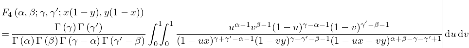
6: 16.15 Integral Representations and Integrals

… ►

16.15.1 $$F_1(\alpha ;\beta ,{\beta }^{\prime };\gamma ;x,y)=\frac{\mathrm{\Gamma }\left(\gamma \right)}{\mathrm{\Gamma }\left(\alpha \right)\mathrm{\Gamma }\left(\gamma -\alpha \right)}{\int }_0^1\frac{u^{\alpha -1}{(1-u)}^{\gamma -\alpha -1}}{{(1-ux)}^{\beta }{(1-uy)}^{{\beta }^{\prime }}}du,$$ $\mathrm{\Re }\alpha >0$, $\mathrm{\Re }\left(\gamma -\alpha \right)>0$,

ⓘ

Symbols:

$F_1(\alpha ;\beta ,{\beta }^{\prime };\gamma ;x,y)$: first Appell function, $\mathrm{\Gamma }\left(z\right)$: gamma function, $dx$: differential of $x$ , $\int$: integral and $\mathrm{\Re }$: real part

Keywords:

Mellin transform

Permalink:

http://dlmf.nist.gov/16.15.E1

Encodings:

pMML, png, TeX

See also:

Annotations for §16.15 and Ch.16

►

16.15.2 $$F_2(\alpha ;\beta ,{\beta }^{\prime };\gamma ,{\gamma }^{\prime };x,y)=\frac{\mathrm{\Gamma }\left(\gamma \right)\mathrm{\Gamma }\left({\gamma }^{\prime }\right)}{\mathrm{\Gamma }\left(\beta \right)\mathrm{\Gamma }\left({\beta }^{\prime }\right)\mathrm{\Gamma }\left(\gamma -\beta \right)\mathrm{\Gamma }\left({\gamma }^{\prime }-{\beta }^{\prime }\right)}{\int }_0^1{\int }_0^1\frac{u^{\beta -1}{v}^{{\beta }^{\prime }-1}{(1-u)}^{\gamma -\beta -1}{(1-v)}^{{\gamma }^{\prime }-{\beta }^{\prime }-1}}{{(1-ux-vy)}^{\alpha }}dudv,$$ $\mathrm{\Re }\gamma >\mathrm{\Re }\beta >0$, $\mathrm{\Re }{\gamma }^{\prime }>\mathrm{\Re }{\beta }^{\prime }>0$,

ⓘ

Symbols:

$F_2(\alpha ;\beta ,{\beta }^{\prime };\gamma ,{\gamma }^{\prime };x,y)$: second Appell function, $\mathrm{\Gamma }\left(z\right)$: gamma function, $dx$: differential of $x$ , $\int$: integral and $\mathrm{\Re }$: real part

Keywords:

Mellin transform

Permalink:

http://dlmf.nist.gov/16.15.E2

Encodings:

pMML, png, TeX

See also:

Annotations for §16.15 and Ch.16

►

16.15.3 $$F_3(\alpha ,{\alpha }^{\prime };\beta ,{\beta }^{\prime };\gamma ;x,y)=\frac{\mathrm{\Gamma }\left(\gamma \right)}{\mathrm{\Gamma }\left(\beta \right)\mathrm{\Gamma }\left({\beta }^{\prime }\right)\mathrm{\Gamma }\left(\gamma -\beta -{\beta }^{\prime }\right)}{\iint }_{\mathrm{\Delta }}\frac{u^{\beta -1}{v}^{{\beta }^{\prime }-1}{(1-u-v)}^{\gamma -\beta -{\beta }^{\prime }-1}}{{(1-ux)}^{\alpha }{(1-vy)}^{{\alpha }^{\prime }}}dudv,$$ $\mathrm{\Re }\left(\gamma -\beta -{\beta }^{\prime }\right)>0$, $\mathrm{\Re }\beta >0$, $\mathrm{\Re }{\beta }^{\prime }>0$,

ⓘ

Symbols:

$F_3(\alpha ,{\alpha }^{\prime };\beta ,{\beta }^{\prime };\gamma ;x,y)$: third Appell function, $\mathrm{\Gamma }\left(z\right)$: gamma function, $dx$: differential of $x$ and $\mathrm{\Re }$: real part

Keywords:

Mellin transform

Notes:

Erdélyi et al. (1953a, 5.8.1(3)) contains a typo.

Referenced by:

Erratum (V1.0.14) for Equation (16.15.3), Erratum (V1.0.14) for Equation (16.15.3)

Permalink:

http://dlmf.nist.gov/16.15.E3

Encodings:

pMML, png, TeX

Clarification (effective with 1.0.14):

A stray “$f$” was removed; it appeared after the comma at the end of this equation.

See also:

Annotations for §16.15 and Ch.16

… ►

16.15.4 $$F_4(\alpha ,\beta ;\gamma ,{\gamma }^{\prime };x(1-y),y(1-x))=\frac{\mathrm{\Gamma }\left(\gamma \right)\mathrm{\Gamma }\left({\gamma }^{\prime }\right)}{\mathrm{\Gamma }\left(\alpha \right)\mathrm{\Gamma }\left(\beta \right)\mathrm{\Gamma }\left(\gamma -\alpha \right)\mathrm{\Gamma }\left({\gamma }^{\prime }-\beta \right)}{\int }_0^1{\int }_0^1\frac{u^{\alpha -1}{v}^{\beta -1}{(1-u)}^{\gamma -\alpha -1}{(1-v)}^{{\gamma }^{\prime }-\beta -1}}{{(1-ux)}^{\gamma +{\gamma }^{\prime }-\alpha -1}{(1-vy)}^{\gamma +{\gamma }^{\prime }-\beta -1}{(1-ux-vy)}^{\alpha +\beta -\gamma -{\gamma }^{\prime }+1}}dudv,$$ $\mathrm{\Re }\gamma >\mathrm{\Re }\alpha >0$, $\mathrm{\Re }{\gamma }^{\prime }>\mathrm{\Re }\beta >0$.

ⓘ

Symbols:

$F_4(\alpha ,\beta ;\gamma ,{\gamma }^{\prime };x,y)$: fourth Appell function, $\mathrm{\Gamma }\left(z\right)$: gamma function, $dx$: differential of $x$ , $\int$: integral and $\mathrm{\Re }$: real part

Keywords:

Mellin transform

Source:

Burchnall and Chaundy (1940, (68))

Referenced by:

§16.15

Permalink:

http://dlmf.nist.gov/16.15.E4

Encodings:

pMML, png, TeX

See also:

Annotations for §16.15 and Ch.16

…

7: 32.9 Other Elementary Solutions

… ►with $\kappa$, $\lambda$, $\mu$, and $\nu$ arbitrary constants. … ►with $C$ an arbitrary constant, which is solvable by quadrature. … ►with $\kappa$ and $\mu$ arbitrary constants. … ►with $C$ an arbitrary constant, which is solvable by quadrature. … ►with $\kappa$ and $\mu$ arbitrary constants. …

8: 5.17 Barnes’ $G$-Function (Double Gamma Function)

… ►

$G\left(z+1\right)=\mathrm{\Gamma }\left(z\right)G\left(z\right),$

… ►Here $B_{2k+2}$ is the Bernoulli number (§24.2(i)), and $A$ is Glaisher’s constant, given by ►

5.17.6 $$A={\mathrm{e}}^C=\mathrm{1.28242\hspace{0.33em}71291\hspace{0.33em}00622\hspace{0.33em}63687}\mathrm{\dots },$$

ⓘ

Symbols:

$\mathrm{e}$: base of natural logarithm, $A$: Glaisher’s constant and $C$: log of Glaisher’s Constant

Notes:

For more digits see OEIS Sequence A074962; see also Sloane (2003).

Permalink:

http://dlmf.nist.gov/5.17.E6

Encodings:

pMML, png, TeX

See also:

Annotations for §5.17 and Ch.5

… ►

5.17.7 $$C=\underset{n\to \mathrm{\infty }}{lim}\left(\sum _{k=1}^{n}k\ln k-\left(\frac{1}{2}{n}^2+\frac{1}{2}n+\frac{1}{12}\right)\ln n+\frac{1}{4}{n}^2\right)=\frac{\gamma +\ln \left(2\pi \right)}{12}-\frac{{\zeta }^{\prime }\left(2\right)}{2{\pi }^2}=\frac{1}{12}-{\zeta }^{\prime }\left(-1\right),$$

ⓘ

Symbols:

$\gamma$: Euler’s constant, $\zeta \left(s\right)$: Riemann zeta function, $\pi$: the ratio of the circumference of a circle to its diameter, $\ln z$: principal branch of logarithm function, $n$: nonnegative integer, $k$: nonnegative integer and $C$: log of Glaisher’s Constant

Referenced by:

§5.17

Permalink:

http://dlmf.nist.gov/5.17.E7

Encodings:

pMML, png, TeX

See also:

Annotations for §5.17 and Ch.5

… ►For Glaisher’s constant see also Greene and Knuth (1982, p. 100) and §2.10(i).

9: 30.5 Functions of the Second Kind

… ►Other solutions of (30.2.1) with $\mu =m$, $\lambda ={\lambda }_n^m\left({\gamma }^2\right)$, and $z=x$ are ►

30.5.1 $${\mathrm{𝖰𝗌}}_n^m(x,{\gamma }^2),$$ $n=m,m+1,m+2,\mathrm{\dots }$.

ⓘ

Symbols:

${\mathrm{𝖰𝗌}}_n^m(x,{\gamma }^2)$: spheroidal wave function of the second kind, $x$: real variable, $m$: nonnegative integer, $n\ge m$: integer degree and ${\gamma }^2$: real parameter

Permalink:

http://dlmf.nist.gov/30.5.E1

Encodings:

pMML, png, TeX

See also:

Annotations for §30.5 and Ch.30

… ►

30.5.2 $${\mathrm{𝖰𝗌}}_n^m(-x,{\gamma }^2)={(-1)}^{n-m+1}{\mathrm{𝖰𝗌}}_n^m(x,{\gamma }^2),$$

ⓘ

Symbols:

${\mathrm{𝖰𝗌}}_n^m(x,{\gamma }^2)$: spheroidal wave function of the second kind, $x$: real variable, $m$: nonnegative integer, $n\ge m$: integer degree and ${\gamma }^2$: real parameter

Permalink:

http://dlmf.nist.gov/30.5.E2

Encodings:

pMML, png, TeX

See also:

Annotations for §30.5 and Ch.30

… ►

30.5.4 $$𝒲\left\{{\mathrm{𝖯𝗌}}_n^m(x,{\gamma }^2),{\mathrm{𝖰𝗌}}_n^m(x,{\gamma }^2)\right\}=\frac{(n+m)!}{(1-x^2)(n-m)!}{A}_n^m({\gamma }^2)A_n^{-m}({\gamma }^2)(\ne 0),$$

ⓘ

Symbols:

$𝒲$: Wronskian, $!$: factorial (as in $n!$), ${\mathrm{𝖯𝗌}}_n^m(x,{\gamma }^2)$: spheroidal wave function of the first kind, ${\mathrm{𝖰𝗌}}_n^m(x,{\gamma }^2)$: spheroidal wave function of the second kind, $x$: real variable, $m$: nonnegative integer, $n\ge m$: integer degree, $A_n^m({\gamma }^2)$ and ${\gamma }^2$: real parameter

Permalink:

http://dlmf.nist.gov/30.5.E4

Encodings:

pMML, png, TeX

See also:

Annotations for §30.5 and Ch.30

►with $A_n^{\pm m}({\gamma }^2)$ as in (30.11.4). …

10: 16.16 Transformations of Variables

… ►

16.16.5 $$F_3(\alpha ,\gamma -\alpha ;\beta ,\gamma -\beta ;\gamma ;x,y)={(1-y)}^{\alpha +\beta -\gamma }{}_2{}^{}F_1^{}(\genfrac{}{}{0pt}{}{\alpha ,\beta }{\gamma };x+y-xy),$$

ⓘ

Symbols:

$F_3(\alpha ,{\alpha }^{\prime };\beta ,{\beta }^{\prime };\gamma ;x,y)$: third Appell function and ${}_2{}^{}F_1^{}(a,b;c;z)$: $=F(a,b;c;z)$ notation for Gauss’ hypergeometric function

Permalink:

http://dlmf.nist.gov/16.16.E5

Encodings:

pMML, png, TeX

See also:

Annotations for §16.16(i), §16.16 and Ch.16

►

16.16.5_5 $$F_4(\alpha ,\beta ;\gamma ,\beta ;x(1-y),y(1-x))={(1-x)}^{-\alpha }{(1-y)}^{-\alpha }{F}_1(\alpha ;\gamma -\beta ,\alpha -\gamma +1;\gamma ;\frac{x}{x-1},\frac{xy}{(1-x)(1-y)}),$$

ⓘ

Symbols:

$F_1(\alpha ;\beta ,{\beta }^{\prime };\gamma ;x,y)$: first Appell function and $F_4(\alpha ,\beta ;\gamma ,{\gamma }^{\prime };x,y)$: fourth Appell function

Referenced by:

§16.16(i), Erratum (V1.1.12) for Additions

Permalink:

http://dlmf.nist.gov/16.16.E5_5

Encodings:

pMML, png, TeX

Addition (effective with 1.1.12):

This equation was added.

See also:

Annotations for §16.16(i), §16.16 and Ch.16

… ►

16.16.7 $$F_4(\alpha ,\beta ;\gamma ,{\gamma }^{\prime };x(1-y),y(1-x))=\sum _{k=0}^{\mathrm{\infty }}\frac{{\left(\alpha \right)}_k{\left(\beta \right)}_k{\left(\alpha +\beta -\gamma -{\gamma }^{\prime }+1\right)}_k}{{\left(\gamma \right)}_k{\left({\gamma }^{\prime }\right)}_{k}k!}{x}^k{y}^k{}_2{}^{}F_1^{}(\genfrac{}{}{0pt}{}{\alpha +k,\beta +k}{\gamma +k};x){}_2{}^{}F_1^{}(\genfrac{}{}{0pt}{}{\alpha +k,\beta +k}{{\gamma }^{\prime }+k};y);$$

ⓘ

Symbols:

$F_4(\alpha ,\beta ;\gamma ,{\gamma }^{\prime };x,y)$: fourth Appell function, ${}_2{}^{}F_1^{}(a,b;c;z)$: $=F(a,b;c;z)$ notation for Gauss’ hypergeometric function, ${\left(a\right)}_n$: Pochhammer’s symbol (or shifted factorial) and $!$: factorial (as in $n!$)

Permalink:

http://dlmf.nist.gov/16.16.E7

Encodings:

pMML, png, TeX

See also:

Annotations for §16.16(i), §16.16 and Ch.16

… ►

16.16.9 $$F_2(\alpha ;\beta ,{\beta }^{\prime };\gamma ,{\gamma }^{\prime };x,y)={(1-x)}^{-\alpha }{F}_2(\alpha ;\gamma -\beta ,{\beta }^{\prime };\gamma ,{\gamma }^{\prime };\frac{x}{x-1},\frac{y}{1-x}),$$

ⓘ

Symbols:

$F_2(\alpha ;\beta ,{\beta }^{\prime };\gamma ,{\gamma }^{\prime };x,y)$: second Appell function

Permalink:

http://dlmf.nist.gov/16.16.E9

Encodings:

pMML, png, TeX

See also:

Annotations for §16.16(ii), §16.16 and Ch.16

►

16.16.10 $$F_4(\alpha ,\beta ;\gamma ,{\gamma }^{\prime };x,y)=\frac{\mathrm{\Gamma }\left({\gamma }^{\prime }\right)\mathrm{\Gamma }\left(\beta -\alpha \right)}{\mathrm{\Gamma }\left({\gamma }^{\prime }-\alpha \right)\mathrm{\Gamma }\left(\beta \right)}{(-y)}^{-\alpha }{F}_4(\alpha ,\alpha -{\gamma }^{\prime }+1;\gamma ,\alpha -\beta +1;\frac{x}{y},\frac{1}{y})+\frac{\mathrm{\Gamma }\left({\gamma }^{\prime }\right)\mathrm{\Gamma }\left(\alpha -\beta \right)}{\mathrm{\Gamma }\left({\gamma }^{\prime }-\beta \right)\mathrm{\Gamma }\left(\alpha \right)}{(-y)}^{-\beta }{F}_4(\beta ,\beta -{\gamma }^{\prime }+1;\gamma ,\beta -\alpha +1;\frac{x}{y},\frac{1}{y}).$$

ⓘ

Symbols:

$F_4(\alpha ,\beta ;\gamma ,{\gamma }^{\prime };x,y)$: fourth Appell function and $\mathrm{\Gamma }\left(z\right)$: gamma function

Permalink:

http://dlmf.nist.gov/16.16.E10

Encodings:

pMML, png, TeX

See also:

Annotations for §16.16(ii), §16.16 and Ch.16

…