Riemann%E2%80%93Siegel%20formula
(0.002 seconds)
1—10 of 351 matching pages
1: 21.7 Riemann Surfaces
§21.7 Riemann Surfaces
►§21.7(i) Connection of Riemann Theta Functions to Riemann Surfaces
►In almost all applications, a Riemann theta function is associated with a compact Riemann surface. … ►is a Riemann matrix and it is used to define the corresponding Riemann theta function. … ►§21.7(iii) Frobenius’ Identity
…2: 25.1 Special Notation
…
►
►
►The main function treated in this chapter is the Riemann zeta function .
This notation was introduced in Riemann (1859).
►The main related functions are the Hurwitz zeta function , the dilogarithm , the polylogarithm (also known as Jonquière’s function ), Lerch’s transcendent , and the Dirichlet -functions .
| nonnegative integers. | |
| … | |
3: 21.2 Definitions
…
►
§21.2(i) Riemann Theta Functions
… ►For numerical purposes we use the scaled Riemann theta function , defined by (Deconinck et al. (2004)), …Many applications involve quotients of Riemann theta functions: the exponential factor then disappears. … ►§21.2(ii) Riemann Theta Functions with Characteristics
… ►It is a translation of the Riemann theta function (21.2.1), multiplied by an exponential factor: …4: 25.10 Zeros
…
►
…
►
§25.10(ii) Riemann–Siegel Formula
… ►Sign changes of are determined by multiplying (25.9.3) by to obtain the Riemann–Siegel formula: … ►Calculations based on the Riemann–Siegel formula reveal that the first ten billion zeros of in the critical strip are on the critical line (van de Lune et al. (1986)). … ►For further information on the Riemann–Siegel expansion see Berry (1995).5: 25.20 Approximations
…
►
•
►
•
►
•
…
►
•
Cody et al. (1971) gives rational approximations for in the form of quotients of polynomials or quotients of Chebyshev series. The ranges covered are , , , . Precision is varied, with a maximum of 20S.
Piessens and Branders (1972) gives the coefficients of the Chebyshev-series expansions of and , , for (23D).
6: 25.18 Methods of Computation
…
►
§25.18(i) Function Values and Derivatives
►The principal tools for computing are the expansion (25.2.9) for general values of , and the Riemann–Siegel formula (25.10.3) (extended to higher terms) for . …Calculations relating to derivatives of and/or can be found in Apostol (1985a), Choudhury (1995), Miller and Adamchik (1998), and Yeremin et al. (1988). … ►§25.18(ii) Zeros
►Most numerical calculations of the Riemann zeta function are concerned with locating zeros of in an effort to prove or disprove the Riemann hypothesis, which states that all nontrivial zeros of lie on the critical line . …7: 21.6 Products
§21.6 Products
►§21.6(i) Riemann Identity
… ►Then …This is the Riemann identity. … ►§21.6(ii) Addition Formulas
…8: 25.4 Reflection Formulas
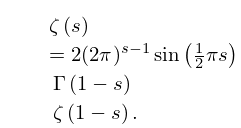
§25.4 Reflection Formulas
… ►
25.4.1
►
25.4.2
…
►
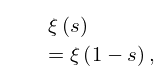
25.4.3
►where is Riemann’s -function, defined by:
…
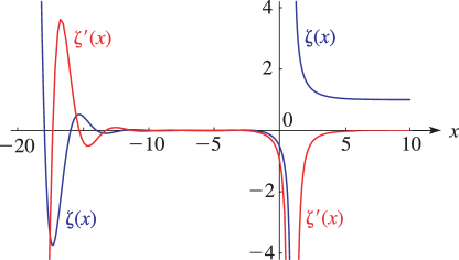
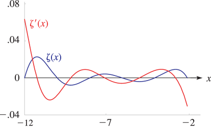
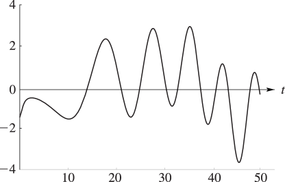
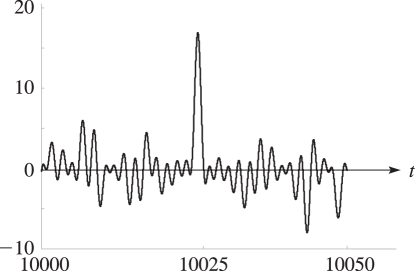
9: 25.3 Graphics
§25.3 Graphics
► ►
►
 ►
►
 ►
►
 ►
►
10: 21.10 Methods of Computation
…
►
•
►
•
►
•
§21.10(i) General Riemann Theta Functions
… ►§21.10(ii) Riemann Theta Functions Associated with a Riemann Surface
… ►Tretkoff and Tretkoff (1984). Here a Hurwitz system is chosen to represent the Riemann surface.
Deconinck and van Hoeij (2001). Here a plane algebraic curve representation of the Riemann surface is used.
