Riemann zeta function

AdvancedHelp

(0.004 seconds)

1—10 of 60 matching pages

1: 25.1 Special Notation
… ► ►►
k , m , n nonnegative integers.
…
►The main function treated in this chapter is the Riemann zeta function ζ ⁡ ( s ) . … ►The main related functions are the Hurwitz zeta function ζ ⁡ ( s , a ) , the dilogarithm Li 2 ⁡ ( z ) , the polylogarithm Li s ⁡ ( z ) (also known as Jonquière’s function ϕ ⁡ ( z , s ) ), Lerch’s transcendent Φ ⁡ ( z , s , a ) , and the Dirichlet L -functions L ⁡ ( s , χ ) .
2: 8.22 Mathematical Applications
… ►
§8.22(ii) Riemann Zeta Function and Incomplete Riemann Zeta Function
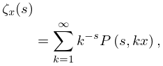
… ►If ζ x ⁡ ( s ) denotes the incomplete Riemann zeta function defined by …so that lim x → ∞ ζ x ⁡ ( s ) = ζ ⁡ ( s ) , then ►
8.22.3 ζ x ⁡ ( s ) = ∑ k = 1 ∞ k − s ⁢ P ⁡ ( s , k ⁢ x ) , ℜ ⁡ s > 1 .
►For further information on ζ x ⁡ ( s ) , including zeros and uniform asymptotic approximations, see Kölbig (1970, 1972a) and Dunster (2006). …
3: 25.7 Integrals
§25.7 Integrals
►For definite integrals of the Riemann zeta function see Prudnikov et al. (1986b, §2.4), Prudnikov et al. (1992a, §3.2), and Prudnikov et al. (1992b, §3.2).
4: 25.17 Physical Applications
§25.17 Physical Applications
… ►See Armitage (1989), Berry and Keating (1998, 1999), Keating (1993, 1999), and Sarnak (1999). …
5: 25.20 Approximations
… ►
  • •

    Cody et al. (1971) gives rational approximations for ζ ⁡ ( s ) in the form of quotients of polynomials or quotients of Chebyshev series. The ranges covered are 0.5 ≤ s ≤ 5 , 5 ≤ s ≤ 11 , 11 ≤ s ≤ 25 , 25 ≤ s ≤ 55 . Precision is varied, with a maximum of 20S.

  • ►
  • •

    Piessens and Branders (1972) gives the coefficients of the Chebyshev-series expansions of s ⁢ ζ ⁡ ( s + 1 ) and ζ ⁡ ( s + k ) , k = 2 , 3 , 4 , 5 , 8 , for 0 ≤ s ≤ 1 (23D).

  • … ►
  • •

    Antia (1993) gives minimax rational approximations for Γ ⁡ ( s + 1 ) ⁢ F s ⁡ ( x ) , where F s ⁡ ( x ) is the Fermi–Dirac integral (25.12.14), for the intervals − ∞ < x ≤ 2 and 2 ≤ x < ∞ , with s = − 1 2 , 1 2 , 3 2 , 5 2 . For each s there are three sets of approximations, with relative maximum errors 10 − 4 , 10 − 8 , 10 − 12 .

  • 6: 25.3 Graphics
    §25.3 Graphics
    ►
    ►See accompanying text►
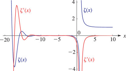
    Figure 25.3.1: Riemann zeta function ζ ⁡ ( x ) and its derivative ζ ′ ⁡ ( x ) , − 20 ≤ x ≤ 10 . Magnify
    ►
    ►See accompanying text►
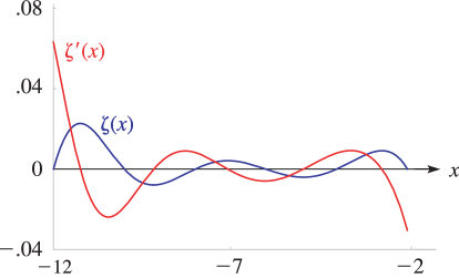
    Figure 25.3.2: Riemann zeta function ζ ⁡ ( x ) and its derivative ζ ′ ⁡ ( x ) , − 12 ≤ x ≤ − 2 . Magnify
    ►
    ►
    See accompanying text
    ►
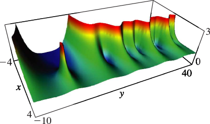
    Figure 25.3.3: Modulus of the Riemann zeta function | ζ ⁡ ( x + i ⁢ y ) | , − 4 ≤ x ≤ 4 , − 10 ≤ y ≤ 40 . Magnify 3D Help
    … ►
    ►See accompanying text►
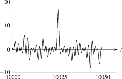
    Figure 25.3.6: Z ⁡ ( t ) , 10000 ≤ t ≤ 10050 . Magnify
    7: 25.18 Methods of Computation
    … ►
    §25.18(i) Function Values and Derivatives
    … ►Calculations relating to derivatives of ζ ⁡ ( s ) and/or ζ ⁡ ( s , a ) can be found in Apostol (1985a), Choudhury (1995), Miller and Adamchik (1998), and Yeremin et al. (1988). … ►
    §25.18(ii) Zeros
    ►Most numerical calculations of the Riemann zeta function are concerned with locating zeros of ζ ⁡ ( 1 2 + i ⁢ t ) in an effort to prove or disprove the Riemann hypothesis, which states that all nontrivial zeros of ζ ⁡ ( s ) lie on the critical line ℜ ⁡ s = 1 2 . …
    8: 27.4 Euler Products and Dirichlet Series
    … ►The completely multiplicative function f ⁡ ( n ) = n − s gives the Euler product representation of the Riemann zeta function ζ ⁡ ( s ) (§25.2(i)): … ►The Riemann zeta function is the prototype of series of the form … ►
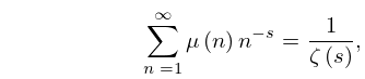
    27.4.5 ∑ n = 1 ∞ μ ⁡ ( n ) ⁢ n − s = 1 ζ ⁡ ( s ) , ℜ ⁡ s > 1 ,
    … ►
    27.4.7 ∑ n = 1 ∞ λ ⁡ ( n ) ⁢ n − s = ζ ⁡ ( 2 ⁢ s ) ζ ⁡ ( s ) , ℜ ⁡ s > 1 ,
    … ►
    27.4.12 ∑ n = 1 ∞ Λ ⁡ ( n ) ⁢ n − s = − ζ ′ ⁡ ( s ) ζ ⁡ ( s ) , ℜ ⁡ s > 1 ,
    …
    9: 25.4 Reflection Formulas
    §25.4 Reflection Formulas
    … ►
    25.4.1 ζ ⁡ ( 1 − s ) = 2 ⁢ ( 2 ⁢ π ) − s ⁢ cos ⁡ ( 1 2 ⁢ π ⁢ s ) ⁢ Γ ⁡ ( s ) ⁢ ζ ⁡ ( s ) ,
    ►
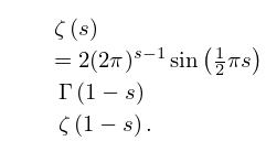
    25.4.2 ζ ⁡ ( s ) = 2 ⁢ ( 2 ⁢ π ) s − 1 ⁢ sin ⁡ ( 1 2 ⁢ π ⁢ s ) ⁢ Γ ⁡ ( 1 − s ) ⁢ ζ ⁡ ( 1 − s ) .
    … ►
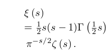
    25.4.4 ξ ⁡ ( s ) = 1 2 ⁢ s ⁢ ( s − 1 ) ⁢ Γ ⁡ ( 1 2 ⁢ s ) ⁢ π − s / 2 ⁢ ζ ⁡ ( s ) .
    … ►
    25.4.5 ( − 1 ) k ⁢ ζ ( k ) ⁡ ( 1 − s ) = 2 ( 2 ⁢ π ) s ⁢ ∑ m = 0 k ∑ r = 0 m ( k m ) ⁢ ( m r ) ⁢ ( ℜ ⁡ ( c k − m ) ⁢ cos ⁡ ( 1 2 ⁢ π ⁢ s ) + ℑ ⁡ ( c k − m ) ⁢ sin ⁡ ( 1 2 ⁢ π ⁢ s ) ) ⁢ Γ ( r ) ⁡ ( s ) ⁢ ζ ( m − r ) ⁡ ( s ) ,
    …
    10: 25.8 Sums
    §25.8 Sums
    ►
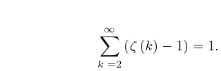
    25.8.1 ∑ k = 2 ∞ ( ζ ⁡ ( k ) − 1 ) = 1 .
    ►
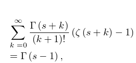
    25.8.2 ∑ k = 0 ∞ Γ ⁡ ( s + k ) ( k + 1 ) ! ⁢ ( ζ ⁡ ( s + k ) − 1 ) = Γ ⁡ ( s − 1 ) , s ≠ 1 , 0 , − 1 , − 2 , … .
    … ►
    25.8.4 ∑ k = 1 ∞ ( − 1 ) k k ⁢ ( ζ ⁡ ( n ⁢ k ) − 1 ) = ln ⁡ ( ∏ j = 0 n − 1 Γ ⁡ ( 2 − e ( 2 ⁢ j + 1 ) ⁢ π ⁢ i / n ) ) , n = 2 , 3 , 4 , … .
    … ►
    25.8.9 ∑ k = 1 ∞ ζ ⁡ ( 2 ⁢ k ) ( 2 ⁢ k + 1 ) ⁢ 2 2 ⁢ k = 1 2 − 1 2 ⁢ ln ⁡ 2 .
    …