Pochhammer%20double-loop%20contour

(0.004 seconds)

1—10 of 260 matching pages

1: 31.9 Orthogonality

… ►

31.9.2

\int_{\zeta}^{(1+,0+,1-,0-)}t^{\gamma-1}(1-t)^{\delta-1}(t-a)^{\epsilon-1}\*w_% {m}(t)w_{k}(t)\,\mathrm{d}t=\delta_{m,k}\theta_{m}.

ⓘ

Symbols:: $\delta_{\NVar{j},\NVar{k}}$ : Kronecker delta, $\,\mathrm{d}\NVar{x}$ : differential of $x$ , $\int$ : integral, $\gamma$ : real or complex parameter, $\delta$ : real or complex parameter, $\epsilon$ : real or complex parameter, $m$ : nonnegative integer, $a$ : complex parameter, $\zeta$ : point and $\theta_{m}$ : normalization constant
Permalink:: http://dlmf.nist.gov/31.9.E2
Encodings:: pMML, png, TeX
See also:: Annotations for §31.9(i), §31.9 and Ch.31

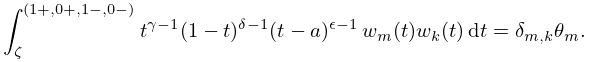
… ►The integration path is called a Pochhammer double-loop contour (compare Figure 5.12.3). … ►and the integration paths

\mathcal{L}_{1}

\mathcal{L}_{2}

are Pochhammer double-loop contours encircling distinct pairs of singularities

\{0,1\}

\{0,a\}

\{1,a\}

. …

2: 13.4 Integral Representations

… ►

§13.4(ii) Contour Integrals

… ►

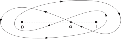
See accompanying text — Figure 13.4.1: Contour of integration in (13.4.11). … Magnify

… ►The contour of integration starts and terminates at a point

\alpha

on the real axis between

0

and

1

. …The contour cuts the real axis between

-1

and

0

. … ►

3: 15.6 Integral Representations

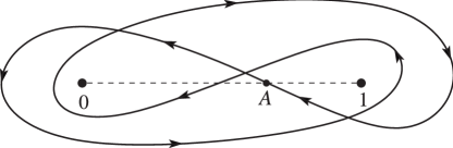
… ►In (15.6.3) the point

\ifrac{1}{(z-1)}

lies outside the integration contour, the contour cuts the real axis between

t=-1

and

0

, at which point

\operatorname{ph}t=\pi

and

\operatorname{ph}\left(1+t\right)=0

. ►In (15.6.4) the point

\ifrac{1}{z}

lies outside the integration contour, and at the point where the contour cuts the negative real axis

\operatorname{ph}t=\pi

and

\operatorname{ph}\left(1-t\right)=0

. ►In (15.6.5) the integration contour starts and terminates at a point

A

on the real axis between

0

and

1

. …However, this reverses the direction of the integration contour, and in consequence (15.6.5) would need to be multiplied by

-1

. … ►

4: 31.10 Integral Equations and Representations

… ►for a suitable contour

C

. …The contour

C

must be such that … ►where

\Re\gamma>0

\Re\delta>0

, and

C

be the Pochhammer double-loop contour about 0 and 1 (as in §31.9(i)). … ►for suitable contours

C_{1}

C_{2}

. …The contours

C_{1}

C_{2}

must be chosen so that …

5: 20 Theta Functions

Chapter 20 Theta Functions

…

6: 17.6 ${{}_{2}\phi_{1}}$ Function

… ►

17.6.4

{{}_{2}\phi_{1}}\left({b^{2},\ifrac{b^{2}}{c}\atop c};q^{2},\ifrac{cq}{b^{2}}% \right)=\frac{1}{2}\frac{\left(b^{2},q;q^{2}\right)_{\infty}}{\left(c,cq/b^{2}% ;q^{2}\right)_{\infty}}\left(\frac{\left(c/b;q\right)_{\infty}}{\left(b;q% \right)_{\infty}}+\frac{\left(-c/b;q\right)_{\infty}}{\left(-b;q\right)_{% \infty}}\right),

|cq|<|b^{2}|

ⓘ

Symbols:: $\left(\NVar{a};\NVar{q}\right)_{\NVar{n}}$ : $q$ -Pochhammer symbol (or $q$ -shifted factorial), ${{}_{\NVar{r+1}}\phi_{\NVar{s}}}\left(\NVar{a_{0},\dots,a_{r}};\NVar{b_{1},% \dots,b_{s}};\NVar{q},\NVar{z}\right)$ or ${{}_{\NVar{r+1}}\phi_{\NVar{s}}}\left({\NVar{a_{0},\dots,a_{r}}\atop\NVar{b_{1% },\dots,b_{s}}};\NVar{q},\NVar{z}\right)$ : basic hypergeometric (or $q$ -hypergeometric) function, $\left(\NVar{a_{1},a_{2},\dots,a_{r}};\NVar{q}\right)_{\NVar{n}}$ : multiple $q$ -Pochhammer symbol and $q$ : complex base
Referenced by:: §17.7(i), §17.7(i), §17.8
Permalink:: http://dlmf.nist.gov/17.6.E4
Encodings:: pMML, png, TeX
See also:: Annotations for §17.6(i), §17.6(i), §17.6 and Ch.17

… ►

17.6.4_5

{{}_{2}\phi_{1}}\left({b^{2},\ifrac{b^{2}}{c}\atop cq^{2}};q^{2},\ifrac{cq^{3}% }{b^{2}}\right)=\frac{1}{2b}\frac{\left(b^{2},q;q^{2}\right)_{\infty}}{\left(% cq^{2},\ifrac{cq}{b^{2}};q^{2}\right)_{\infty}}\left(\frac{\left(\ifrac{cq}{b}% ;q\right)_{\infty}}{\left(b;q\right)_{\infty}}-\frac{\left(\ifrac{-cq}{b};q% \right)_{\infty}}{\left(-b;q\right)_{\infty}}\right),

\left|cq^{3}\right|<\left|b^{2}\right|

ⓘ

Symbols:: $\left(\NVar{a};\NVar{q}\right)_{\NVar{n}}$ : $q$ -Pochhammer symbol (or $q$ -shifted factorial), ${{}_{\NVar{r+1}}\phi_{\NVar{s}}}\left(\NVar{a_{0},\dots,a_{r}};\NVar{b_{1},% \dots,b_{s}};\NVar{q},\NVar{z}\right)$ or ${{}_{\NVar{r+1}}\phi_{\NVar{s}}}\left({\NVar{a_{0},\dots,a_{r}}\atop\NVar{b_{1% },\dots,b_{s}}};\NVar{q},\NVar{z}\right)$ : basic hypergeometric (or $q$ -hypergeometric) function, $\left(\NVar{a_{1},a_{2},\dots,a_{r}};\NVar{q}\right)_{\NVar{n}}$ : multiple $q$ -Pochhammer symbol and $q$ : complex base
Source:: Verma and Jain (1983, (3.6))
Referenced by:: §17.6(i), Erratum (V1.1.0) for Additions
Permalink:: http://dlmf.nist.gov/17.6.E4_5
Encodings:: pMML, png, TeX
Addition (effective with 1.1.0):: This equation was added.
Suggested 2019-10-19 by Slobodan Damjanovic
See also:: Annotations for §17.6(i), §17.6(i), §17.6 and Ch.17

… ►

17.6.11

\frac{1-z}{1-b}{{}_{2}\phi_{1}}\left({q,aq\atop bq};q,z\right)=\sum_{n=0}^{% \infty}\frac{\left(aq;q\right)_{n}\left(azq/b;q\right)_{2n}b^{n}}{\left(zq,aq/% b;q\right)_{n}}-aq\sum_{n=0}^{\infty}\frac{\left(aq;q\right)_{n}\left(azq/b;q% \right)_{2n+1}(bq)^{n}}{\left(zq;q\right)_{n}\left(aq/b;q\right)_{n+1}},

|z|<1,|b|<1

ⓘ

Symbols:: $\left(\NVar{a};\NVar{q}\right)_{\NVar{n}}$ : $q$ -Pochhammer symbol (or $q$ -shifted factorial), ${{}_{\NVar{r+1}}\phi_{\NVar{s}}}\left(\NVar{a_{0},\dots,a_{r}};\NVar{b_{1},% \dots,b_{s}};\NVar{q},\NVar{z}\right)$ or ${{}_{\NVar{r+1}}\phi_{\NVar{s}}}\left({\NVar{a_{0},\dots,a_{r}}\atop\NVar{b_{1% },\dots,b_{s}}};\NVar{q},\NVar{z}\right)$ : basic hypergeometric (or $q$ -hypergeometric) function, $\left(\NVar{a_{1},a_{2},\dots,a_{r}};\NVar{q}\right)_{\NVar{n}}$ : multiple $q$ -Pochhammer symbol, $q$ : complex base, $n$ : nonnegative integer and $z$ : complex variable
Permalink:: http://dlmf.nist.gov/17.6.E11
Encodings:: pMML, png, TeX
See also:: Annotations for §17.6(ii), §17.6(ii), §17.6 and Ch.17

… ►

17.6.14

\sum_{n=0}^{\infty}\frac{\left(a;q\right)_{n}\left(b;q^{2}\right)_{n}z^{n}}{% \left(q;q\right)_{n}\left(azb;q^{2}\right)_{n}}=\frac{\left(az,bz;q^{2}\right)% _{\infty}}{\left(z,azb;q^{2}\right)_{\infty}}{{}_{2}\phi_{1}}\left({a,b\atop bz% };q^{2},zq\right).

ⓘ

Symbols:: $\left(\NVar{a};\NVar{q}\right)_{\NVar{n}}$ : $q$ -Pochhammer symbol (or $q$ -shifted factorial), ${{}_{\NVar{r+1}}\phi_{\NVar{s}}}\left(\NVar{a_{0},\dots,a_{r}};\NVar{b_{1},% \dots,b_{s}};\NVar{q},\NVar{z}\right)$ or ${{}_{\NVar{r+1}}\phi_{\NVar{s}}}\left({\NVar{a_{0},\dots,a_{r}}\atop\NVar{b_{1% },\dots,b_{s}}};\NVar{q},\NVar{z}\right)$ : basic hypergeometric (or $q$ -hypergeometric) function, $\left(\NVar{a_{1},a_{2},\dots,a_{r}};\NVar{q}\right)_{\NVar{n}}$ : multiple $q$ -Pochhammer symbol, $q$ : complex base, $n$ : nonnegative integer and $z$ : complex variable
Referenced by:: §17.6(ii)
Permalink:: http://dlmf.nist.gov/17.6.E14
Encodings:: pMML, png, TeX
See also:: Annotations for §17.6(ii), §17.6(ii), §17.6 and Ch.17

… ►where

|z|<1

|\operatorname{ph}\left(-z\right)|<\pi

, and the contour of integration separates the poles of

\left(q^{1+\zeta},cq^{\zeta};q\right)_{\infty}/\sin\left(\pi\zeta\right)

from those of

1/\left(aq^{\zeta},bq^{\zeta};q\right)_{\infty}

, and the infimum of the distances of the poles from the contour is positive. …

7: 18.5 Explicit Representations

… ►

18.5.12

L^{(\alpha)}_{n}\left(x\right)=\sum_{\ell=0}^{n}\frac{{\left(\alpha+\ell+1% \right)_{n-\ell}}}{(n-\ell)!\;\ell!}(-x)^{\ell}=\frac{{\left(\alpha+1\right)_{% n}}}{n!}{{}_{1}F_{1}}\left({-n\atop\alpha+1};x\right).

… ►

T_{5}\left(x\right)=16x^{5}-20x^{3}+5x,

… ►

L_{6}\left(x\right)=\tfrac{1}{720}x^{6}-\tfrac{1}{20}x^{5}+\tfrac{5}{8}x^{4}-% \tfrac{10}{3}x^{3}+\tfrac{15}{2}x^{2}-6x+1.

… ►

L^{(\alpha)}_{3}\left(x\right)=-\tfrac{1}{6}x^{3}+\tfrac{1}{2}(\alpha+3)x^{2}-% \tfrac{1}{2}{\left(\alpha+2\right)_{2}}x+\tfrac{1}{6}{\left(\alpha+1\right)_{3% }},

►

L^{(\alpha)}_{4}\left(x\right)=\tfrac{1}{24}x^{4}-\tfrac{1}{6}(\alpha+4)x^{3}+% \tfrac{1}{4}{\left(\alpha+3\right)_{2}}x^{2}-\tfrac{1}{6}{\left(\alpha+2\right% )_{3}}x+\tfrac{1}{24}{\left(\alpha+1\right)_{4}}.

…

8: 17.14 Constant Term Identities

… ►

17.14.1

\frac{\left(q;q\right)_{a_{1}+a_{2}+\cdots+a_{n}}}{\left(q;q\right)_{a_{1}}% \left(q;q\right)_{a_{2}}\cdots\left(q;q\right)_{a_{n}}}=\mbox{ coeff. of }x_{1% }^{0}x_{2}^{0}\cdots x_{n}^{0}\mbox{ in }\prod_{1\leq j<k\leq n}\left(\frac{x_% {j}}{x_{k}};q\right)_{a_{j}}\left(\frac{qx_{k}}{x_{j}};q\right)_{a_{k}}.

ⓘ

Symbols:: $\left(\NVar{a};\NVar{q}\right)_{\NVar{n}}$ : $q$ -Pochhammer symbol (or $q$ -shifted factorial), $k$ : nonnegative integer, $q$ : complex base, $j$ : nonnegative integer, $n$ : nonnegative integer and $x$ : real variable
Referenced by:: §17.14
Permalink:: http://dlmf.nist.gov/17.14.E1
Encodings:: pMML, png, TeX
See also:: Annotations for §17.14, §17.14 and Ch.17

… ►

17.14.2

\sum_{n=0}^{\infty}\frac{q^{n(n+1)}}{\left(q^{2};q^{2}\right)_{n}\left(-q;q^{2% }\right)_{n+1}}=\mbox{ coeff. of }z^{0}\mbox{ in }\frac{\left(-zq;q^{2}\right)% _{\infty}\left(-z^{-1}q;q^{2}\right)_{\infty}\left(q^{2};q^{2}\right)_{\infty}% }{\left(z^{-1}q^{2};q^{2}\right)_{\infty}\left(-q;q^{2}\right)_{\infty}\left(z% ^{-1}q;q^{2}\right)_{\infty}}=\frac{1}{\left(-q;q^{2}\right)_{\infty}}\mbox{ % coeff. of }z^{0}\mbox{ in }\frac{\left(-zq;q^{2}\right)_{\infty}\left(-z^{-1}q% ;q^{2}\right)_{\infty}\left(q^{2};q^{2}\right)_{\infty}}{\left(z^{-1}q;q\right% )_{\infty}}=\frac{H(q)}{\left(-q;q^{2}\right)_{\infty}},

ⓘ

Symbols:: $\left(\NVar{a};\NVar{q}\right)_{\NVar{n}}$ : $q$ -Pochhammer symbol (or $q$ -shifted factorial), $q$ : complex base, $n$ : nonnegative integer, $z$ : complex variable and $H(q)$ : LHS of (17.2.50)
Referenced by:: §17.14
Permalink:: http://dlmf.nist.gov/17.14.E2
Encodings:: pMML, png, TeX
See also:: Annotations for §17.14, §17.14 and Ch.17

►

17.14.3

\sum_{n=0}^{\infty}\frac{q^{n(n+1)}}{\left(q^{2};q^{2}\right)_{n}\left(-q;q^{2% }\right)_{n+1}}=\mbox{ coeff. of }z^{0}\mbox{ in }\frac{\left(-zq;q^{2}\right)% _{\infty}\left(-z^{-1}q;q^{2}\right)_{\infty}\left(q^{2};q^{2}\right)_{\infty}% }{\left(z^{-1};q^{2}\right)_{\infty}\left(-q;q^{2}\right)_{\infty}\left(z^{-1}% q;q^{2}\right)_{\infty}}=\frac{1}{\left(-q;q^{2}\right)_{\infty}}\mbox{ coeff.% of }z^{0}\mbox{ in }\frac{\left(-zq;q^{2}\right)_{\infty}\left(-z^{-1}q;q^{2}% \right)_{\infty}\left(q^{2};q^{2}\right)_{\infty}}{\left(z^{-1};q\right)_{% \infty}}=\frac{G(q)}{\left(-q;q^{2}\right)_{\infty}},

ⓘ

Symbols:: $\left(\NVar{a};\NVar{q}\right)_{\NVar{n}}$ : $q$ -Pochhammer symbol (or $q$ -shifted factorial), $q$ : complex base, $n$ : nonnegative integer, $z$ : complex variable and $G(q)$ : LHS of (17.2.49)
Permalink:: http://dlmf.nist.gov/17.14.E3
Encodings:: pMML, png, TeX
See also:: Annotations for §17.14, §17.14 and Ch.17

►

17.14.4

\sum_{n=0}^{\infty}\frac{q^{n^{2}}}{\left(q^{2};q^{2}\right)_{n}\left(q;q^{2}% \right)_{n}}=\mbox{ coeff. of }z^{0}\mbox{ in }\frac{\left(-zq;q^{2}\right)_{% \infty}\left(-z^{-1}q;q^{2}\right)_{\infty}\left(q^{2};q^{2}\right)_{\infty}}{% \left(-z^{-1};q^{2}\right)_{\infty}\left(q;q^{2}\right)_{\infty}\left(z^{-1};q% ^{2}\right)_{\infty}}=\frac{1}{\left(q;q^{2}\right)_{\infty}}\mbox{ coeff. of % }z^{0}\mbox{ in }\frac{\left(-zq;q^{2}\right)_{\infty}\left(-z^{-1}q;q^{2}% \right)_{\infty}\left(q^{2};q^{2}\right)_{\infty}}{\left(z^{-2};q^{4}\right)_{% \infty}}=\frac{G(q^{4})}{\left(q;q^{2}\right)_{\infty}},

ⓘ

Symbols:: $\left(\NVar{a};\NVar{q}\right)_{\NVar{n}}$ : $q$ -Pochhammer symbol (or $q$ -shifted factorial), $q$ : complex base, $n$ : nonnegative integer, $z$ : complex variable and $G(q)$ : LHS of (17.2.49)
Permalink:: http://dlmf.nist.gov/17.14.E4
Encodings:: pMML, png, TeX
See also:: Annotations for §17.14, §17.14 and Ch.17

►

17.14.5

\sum_{n=0}^{\infty}\frac{q^{n^{2}+2n}}{\left(q^{2};q^{2}\right)_{n}\left(q;q^{% 2}\right)_{n+1}}=\mbox{ coeff. of }z^{0}\mbox{ in }\frac{\left(-zq;q^{2}\right% )_{\infty}\left(-z^{-1}q;q^{2}\right)_{\infty}\left(q^{2};q^{2}\right)_{\infty% }}{\left(-q^{2}z^{-1};q^{2}\right)_{\infty}\left(q;q^{2}\right)_{\infty}\left(% z^{-1}q^{2};q^{2}\right)_{\infty}}=\frac{1}{\left(q;q^{2}\right)_{\infty}}% \mbox{ coeff. of }z^{0}\mbox{ in }\frac{\left(-zq;q^{2}\right)_{\infty}\left(-% z^{-1}q;q^{2}\right)_{\infty}\left(q^{2};q^{2}\right)_{\infty}}{\left(q^{4}z^{% -2};q^{4}\right)_{\infty}}=\frac{H(q^{4})}{\left(q;q^{2}\right)_{\infty}}.

ⓘ

Symbols:: $\left(\NVar{a};\NVar{q}\right)_{\NVar{n}}$ : $q$ -Pochhammer symbol (or $q$ -shifted factorial), $q$ : complex base, $n$ : nonnegative integer, $z$ : complex variable and $H(q)$ : LHS of (17.2.50)
Referenced by:: §17.14
Permalink:: http://dlmf.nist.gov/17.14.E5
Encodings:: pMML, png, TeX
See also:: Annotations for §17.14, §17.14 and Ch.17

…

9: 16.2 Definition and Analytic Properties

… ►

16.2.1

{{}_{p}F_{q}}\left({a_{1},\dots,a_{p}\atop b_{1},\dots,b_{q}};z\right)=\sum_{k% =0}^{\infty}\frac{{\left(a_{1}\right)_{k}}\cdots{\left(a_{p}\right)_{k}}}{{% \left(b_{1}\right)_{k}}\cdots{\left(b_{q}\right)_{k}}}\frac{z^{k}}{k!}.

ⓘ

Symbols:: ${{}_{\NVar{p}}F_{\NVar{q}}}\left(\NVar{a_{1},\dots,a_{p}};\NVar{b_{1},\dots,b_% {q}};\NVar{z}\right)$ or ${{}_{\NVar{p}}F_{\NVar{q}}}\left({\NVar{a_{1},\dots,a_{p}}\atop\NVar{b_{1},% \dots,b_{q}}};\NVar{z}\right)$ : alternatively ${{}_{\NVar{p}}F_{\NVar{q}}}\left(\NVar{\mathbf{a}};\NVar{\mathbf{b}};\NVar{z}\right)$ or ${{}_{\NVar{p}}F_{\NVar{q}}}\left({\NVar{\mathbf{a}}\atop\NVar{\mathbf{b}}};% \NVar{z}\right)$
generalized hypergeometric function, ${\left(\NVar{a}\right)_{\NVar{n}}}$ : Pochhammer’s symbol (or shifted factorial), $!$ : factorial (as in $n!$ ), $p$ : nonnegative integer, $q$ : nonnegative integer, $z$ : complex variable, $a,a_{1},\ldots,a_{p}$ : real or complex parameters and $b,b_{1},\ldots,b_{q}$ : real or complex parameters
Referenced by:: §10.16, §10.16, §10.39, §16.2(iv), §16.2(ii), §16.2(iii), §16.2(iii), §16.2(iii), §16.5, §18.17(v), §18.17(vi), §18.17(vii), §18.20(ii), §18.26(i), §18.30(i), §18.38(ii)
Permalink:: http://dlmf.nist.gov/16.2.E1
Encodings:: pMML, png, TeX
See also:: Annotations for §16.2(i), §16.2 and Ch.16

… ►

16.2.3

{{}_{p+1}F_{q}}\left({-m,\mathbf{a}\atop\mathbf{b}};z\right)=\frac{{\left(% \mathbf{a}\right)_{m}}(-z)^{m}}{{\left(\mathbf{b}\right)_{m}}}{{}_{q+1}F_{p}}% \left({-m,1-m-\mathbf{b}\atop 1-m-\mathbf{a}};\frac{(-1)^{p+q}}{z}\right)

ⓘ

Symbols:: ${{}_{\NVar{p}}F_{\NVar{q}}}\left(\NVar{a_{1},\dots,a_{p}};\NVar{b_{1},\dots,b_% {q}};\NVar{z}\right)$ or ${{}_{\NVar{p}}F_{\NVar{q}}}\left({\NVar{a_{1},\dots,a_{p}}\atop\NVar{b_{1},% \dots,b_{q}}};\NVar{z}\right)$ : alternatively ${{}_{\NVar{p}}F_{\NVar{q}}}\left(\NVar{\mathbf{a}};\NVar{\mathbf{b}};\NVar{z}\right)$ or ${{}_{\NVar{p}}F_{\NVar{q}}}\left({\NVar{\mathbf{a}}\atop\NVar{\mathbf{b}}};% \NVar{z}\right)$
generalized hypergeometric function, ${\left(\NVar{a}\right)_{\NVar{n}}}$ : Pochhammer’s symbol (or shifted factorial), $p$ : nonnegative integer, $q$ : nonnegative integer and $z$ : complex variable
Referenced by:: §13.6(v)
Permalink:: http://dlmf.nist.gov/16.2.E3
Encodings:: pMML, png, TeX
See also:: Annotations for §16.2(iv), §16.2(iv), §16.2 and Ch.16

… ►

16.2.4

\sum_{k=0}^{m}\frac{{\left(\mathbf{a}\right)_{k}}}{{\left(\mathbf{b}\right)_{k% }}}\frac{z^{k}}{k!}=\frac{{\left(\mathbf{a}\right)_{m}}z^{m}}{{\left(\mathbf{b% }\right)_{m}}m!}{{}_{q+2}F_{p}}\left({-m,1,1-m-\mathbf{b}\atop 1-m-\mathbf{a}}% ;\frac{(-1)^{p+q+1}}{z}\right).

ⓘ

Symbols:: ${{}_{\NVar{p}}F_{\NVar{q}}}\left(\NVar{a_{1},\dots,a_{p}};\NVar{b_{1},\dots,b_% {q}};\NVar{z}\right)$ or ${{}_{\NVar{p}}F_{\NVar{q}}}\left({\NVar{a_{1},\dots,a_{p}}\atop\NVar{b_{1},% \dots,b_{q}}};\NVar{z}\right)$ : alternatively ${{}_{\NVar{p}}F_{\NVar{q}}}\left(\NVar{\mathbf{a}};\NVar{\mathbf{b}};\NVar{z}\right)$ or ${{}_{\NVar{p}}F_{\NVar{q}}}\left({\NVar{\mathbf{a}}\atop\NVar{\mathbf{b}}};% \NVar{z}\right)$
generalized hypergeometric function, ${\left(\NVar{a}\right)_{\NVar{n}}}$ : Pochhammer’s symbol (or shifted factorial), $!$ : factorial (as in $n!$ ), $p$ : nonnegative integer, $q$ : nonnegative integer and $z$ : complex variable
Permalink:: http://dlmf.nist.gov/16.2.E4
Encodings:: pMML, png, TeX
See also:: Annotations for §16.2(iv), §16.2(iv), §16.2 and Ch.16

… ►See §16.5 for the definition of

{{}_{p}F_{q}}\left(\mathbf{a};\mathbf{b};z\right)

as a contour integral when

p>q+1

and none of the

a_{k}

is a nonpositive integer. … ►

16.2.5

{{}_{p}{\mathbf{F}}_{q}}\left(\mathbf{a};\mathbf{b};z\right)=\ifrac{{{}_{p}F_{% q}}\left({a_{1},\dots,a_{p}\atop b_{1},\dots,b_{q}};z\right)}{\left(\Gamma% \left(b_{1}\right)\cdots\Gamma\left(b_{q}\right)\right)}=\sum_{k=0}^{\infty}% \frac{{\left(a_{1}\right)_{k}}\cdots{\left(a_{p}\right)_{k}}}{\Gamma\left(b_{1% }+k\right)\cdots\Gamma\left(b_{q}+k\right)}\frac{z^{k}}{k!};

ⓘ

Defines:: ${{}_{\NVar{p}}{\mathbf{F}}_{\NVar{q}}}\left(\NVar{\mathbf{a}};\NVar{\mathbf{b}% };\NVar{z}\right)$ or ${{}_{\NVar{p}}{\mathbf{F}}_{\NVar{q}}}\left({\NVar{\mathbf{a}}\atop\NVar{% \mathbf{b}}};\NVar{z}\right)$ : scaled (or Olver’s) generalized hypergeometric function
Symbols:: $\Gamma\left(\NVar{z}\right)$ : gamma function, ${{}_{\NVar{p}}F_{\NVar{q}}}\left(\NVar{a_{1},\dots,a_{p}};\NVar{b_{1},\dots,b_% {q}};\NVar{z}\right)$ or ${{}_{\NVar{p}}F_{\NVar{q}}}\left({\NVar{a_{1},\dots,a_{p}}\atop\NVar{b_{1},% \dots,b_{q}}};\NVar{z}\right)$ : alternatively ${{}_{\NVar{p}}F_{\NVar{q}}}\left(\NVar{\mathbf{a}};\NVar{\mathbf{b}};\NVar{z}\right)$ or ${{}_{\NVar{p}}F_{\NVar{q}}}\left({\NVar{\mathbf{a}}\atop\NVar{\mathbf{b}}};% \NVar{z}\right)$
generalized hypergeometric function, ${\left(\NVar{a}\right)_{\NVar{n}}}$ : Pochhammer’s symbol (or shifted factorial), $!$ : factorial (as in $n!$ ), $p$ : nonnegative integer, $q$ : nonnegative integer, $z$ : complex variable, $a,a_{1},\ldots,a_{p}$ : real or complex parameters and $b,b_{1},\ldots,b_{q}$ : real or complex parameters
Referenced by:: §16.2(v)
Permalink:: http://dlmf.nist.gov/16.2.E5
Encodings:: pMML, png, TeX
See also:: Annotations for §16.2(v), §16.2 and Ch.16

…

10: 5.2 Definitions

… ►

§5.2(iii) Pochhammer’s Symbol

►

{\left(a\right)_{0}}=1,

… ►

{\left(a\right)_{2n}}=2^{2n}{\left(\frac{a}{2}\right)_{n}}{\left(\frac{a+1}{2}% \right)_{n}},

►

{\left(a\right)_{2n+1}}=2^{2n+1}{\left(\frac{a}{2}\right)_{n+1}}{\left(\frac{a% +1}{2}\right)_{n}}.

►Pochhammer symbols (rising factorials)

{\left(x\right)_{n}}=x(x+1)\cdots(x+n-1)

and falling factorials

(-1)^{n}{\left(-x\right)_{n}}=x(x-1)\cdots(x-n+1)

can be expressed in terms of each other via …