Picard–Fuchs equations

SearchAdvancedHelp

(0.003 seconds)

1—10 of 450 matching pages

1: 30.2 Differential Equations

§30.2 Differential Equations

►

§30.2(i) Spheroidal Differential Equation

… ► … ►The Liouville normal form of equation (30.2.1) is … ►

§30.2(iii) Special Cases

…

2: 31.2 Differential Equations

§31.2 Differential Equations

►

§31.2(i) Heun’s Equation

►

31.2.1 $$\frac{d^{2}w}{{dz}^2}+\left(\frac{\gamma }{z}+\frac{\delta }{z-1}+\frac{ϵ}{z-a}\right)\frac{dw}{dz}+\frac{\alpha \beta z-q}{z(z-1)(z-a)}w=0,$$ $\alpha +\beta +1=\gamma +\delta +ϵ$.

ⓘ

Symbols:

$\frac{df}{dx}$: derivative of $f$ with respect to $x$ , $z$: complex variable, $\gamma$: real or complex parameter, $\delta$: real or complex parameter, $ϵ$: real or complex parameter, $a$: complex parameter, $q$: real or complex parameter, $\alpha$: real or complex parameter and $\beta$: real or complex parameter

Referenced by:

§29.2(ii), §31.11(iii), §31.12, §31.13, §31.14(i), §31.17(i), §31.18, §31.2(v), §31.2(v), §31.2(v), §31.2(i), §31.3(i), §31.3(i), §31.3(ii), §31.3(ii), §31.3(ii), §31.3(iii), §31.3(iii), §31.4, §31.5, §31.6, §31.7(ii), §31.8, §31.8, §31.8

Permalink:

http://dlmf.nist.gov/31.2.E1

Encodings:

pMML, png, TeX

See also:

Annotations for §31.2(i), §31.2 and Ch.31

… ►

§31.2(v) Heun’s Equation Automorphisms

… ►

Composite Transformations

…

3: 29.2 Differential Equations

§29.2 Differential Equations

►

§29.2(i) Lamé’s Equation

… ►

§29.2(ii) Other Forms

… ►Equation (29.2.10) is a special case of Heun’s equation (31.2.1).

4: 15.10 Hypergeometric Differential Equation

§15.10 Hypergeometric Differential Equation

►

§15.10(i) Fundamental Solutions

►

15.10.1 $$z(1-z)\frac{d^{2}w}{{dz}^2}+\left(c-(a+b+1)z\right)\frac{dw}{dz}-abw=0.$$

ⓘ

Symbols:

$\frac{df}{dx}$: derivative of $f$ with respect to $x$ , $z$: complex variable, $a$: real or complex parameter, $b$: real or complex parameter and $c$: real or complex parameter

Referenced by:

§15.11(i), §15.11(i), §15.17(ii), §15.19(ii), §15.2(ii), §15.5(ii), §16.13, §17.6(iv), §19.18(ii), §19.4(ii)

Permalink:

http://dlmf.nist.gov/15.10.E1

Encodings:

pMML, png, TeX

See also:

Annotations for §15.10(i), §15.10 and Ch.15

►This is the hypergeometric differential equation. … ► …

5: 32.2 Differential Equations

§32.2 Differential Equations

… ►The six Painlevé equations ${\text{P}}_{\text{I}}$–${\text{P}}_{\text{VI}}$ are as follows: … ►

§32.2(ii) Renormalizations

… ► … ►See Fuchs (1907), Painlevé (1906), Gromak et al. (2002, §42); also Manin (1998). …

6: 28.2 Definitions and Basic Properties

… ►

§28.2(i) Mathieu’s Equation

… ►

28.2.1 $$w^{\prime \prime }+(a-2q\cos \left(2z\right))w=0.$$

ⓘ

Symbols:

$\cos z$: cosine function, $q=h^2$: parameter, $z$: complex variable, $a$: parameter and $w(z)$: Mathieu’s equation solution

A&S Ref:

20.3.1 20.1.1 (in slightly different form)

Referenced by:

§1.18(vii), Figure 28.17.1, Figure 28.17.1, §28.17, §28.17, §28.2(ii), §28.2(ii), §28.2(iii), §28.2(iv), §28.20(i), §28.29(i), §28.32(i), §28.32(i), 1st item, 2nd item, §28.33(iii), item (a), item (c), item (c), §28.5(i), §28.8(iv), §28.8(iv), §28.8(iv), §30.2(iii)

Permalink:

http://dlmf.nist.gov/28.2.E1

Encodings:

pMML, png, TeX

See also:

Annotations for §28.2(i), §28.2 and Ch.28

… ►This is the characteristic equation of Mathieu’s equation (28.2.1). … ►

§28.2(iv) Floquet Solutions

… ► …

7: 28.20 Definitions and Basic Properties

… ►

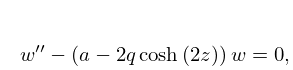
§28.20(i) Modified Mathieu’s Equation

►When $z$ is replaced by $\pm \mathrm{i}z$, (28.2.1) becomes the modified Mathieu’s equation: ►

28.20.1 $$w^{\prime \prime }-\left(a-2q\cosh \left(2z\right)\right)w=0,$$

ⓘ

Symbols:

$\cosh z$: hyperbolic cosine function, $q=h^2$: parameter, $z$: complex variable, $a$: parameter and $w(z)$: Mathieu’s equation solution

A&S Ref:

20.1.2 (in slightly different form) 20.8.6

Referenced by:

§28.20(iii), §28.32(i), 1st item, 2nd item, item (b), §28.8(iv), §28.8(iv)

Permalink:

http://dlmf.nist.gov/28.20.E1

Encodings:

pMML, png, TeX

See also:

Annotations for §28.20(i), §28.20 and Ch.28

… ►

28.20.2 $$({\zeta }^2-1)w^{\prime \prime }+\zeta w^{\prime }+\left(4q{\zeta }^2-2q-a\right)w=0,$$ $\zeta =\cosh z$.

ⓘ

Symbols:

$\cosh z$: hyperbolic cosine function, $q=h^2$: parameter, $z$: complex variable, $a$: parameter and $w(z)$: Mathieu’s equation solution

Referenced by:

§28.20(iii)

Permalink:

http://dlmf.nist.gov/28.20.E2

Encodings:

pMML, png, TeX

See also:

Annotations for §28.20(i), §28.20 and Ch.28

… ►Then from §2.7(ii) it is seen that equation (28.20.2) has independent and unique solutions that are asymptotic to ${\zeta }^{1/2}{\mathrm{e}}^{\pm 2\mathrm{i}h\zeta }$ as $\zeta \to \mathrm{\infty }$ in the respective sectors $|\mathrm{ph}\left(\mp \mathrm{i}\zeta \right)|\le \frac{3}{2}\pi -\delta$, $\delta$ being an arbitrary small positive constant. …

8: 16.23 Mathematical Applications

… ►

§16.23(i) Differential Equations

►A variety of problems in classical mechanics and mathematical physics lead to Picard–Fuchs equations. These equations are frequently solvable in terms of generalized hypergeometric functions, and the monodromy of generalized hypergeometric functions plays an important role in describing properties of the solutions. … …

9: 31.18 Methods of Computation

§31.18 Methods of Computation

►Independent solutions of (31.2.1) can be computed in the neighborhoods of singularities from their Fuchs–Frobenius expansions (§31.3), and elsewhere by numerical integration of (31.2.1). …The computation of the accessory parameter for the Heun functions is carried out via the continued-fraction equations (31.4.2) and (31.11.13) in the same way as for the Mathieu, Lamé, and spheroidal wave functions in Chapters 28–30.

10: 31.3 Basic Solutions

… ►

§31.3(i) Fuchs–Frobenius Solutions at $z=0$

… ►

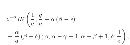
§31.3(ii) Fuchs–Frobenius Solutions at Other Singularities

… ►

31.3.10 $$z^{-\alpha }H\mathrm{\ell }(\frac{1}{a},\frac{q}{a}-\alpha \left(\beta -ϵ\right)-\frac{\alpha }{a}\left(\beta -\delta \right);\alpha ,\alpha -\gamma +1,\alpha -\beta +1,\delta ;\frac{1}{z}),$$

ⓘ

Symbols:

$H\mathrm{\ell }(a,q;\alpha ,\beta ,\gamma ,\delta ;z)$: Heun functions, $z$: complex variable, $\gamma$: real or complex parameter, $\delta$: real or complex parameter, $ϵ$: real or complex parameter, $a$: complex parameter, $q$: real or complex parameter, $\alpha$: real or complex parameter and $\beta$: real or complex parameter

Referenced by:

§31.11(iii), §31.11(iii), Erratum (V1.1.7) for Equations (31.3.10), (31.3.11), Erratum (V1.1.7) for Subsection 31.11(iii)

Permalink:

http://dlmf.nist.gov/31.3.E10

Encodings:

pMML, png, TeX

Correction (effective with 1.1.7):

The second entry in the $H\mathrm{\ell }$ has been corrected with an extra minus sign.

See also:

Annotations for §31.3(ii), §31.3 and Ch.31

… ►

§31.3(iii) Equivalent Expressions

… ►The full set of 192 local solutions of (31.2.1), equivalent in 8 sets of 24, resembles Kummer’s set of 24 local solutions of the hypergeometric equation, which are equivalent in 4 sets of 6 solutions (§15.10(ii)); see Maier (2007).