Legendre functions

SearchAdvancedHelp

(0.009 seconds)

1—10 of 161 matching pages

1: 14.1 Special Notation

§14.1 Special Notation

… ►The main functions treated in this chapter are the Legendre functions ${𝖯}_{\nu }\left(x\right)$, ${𝖰}_{\nu }\left(x\right)$, $P_{\nu }\left(z\right)$, $Q_{\nu }\left(z\right)$; Ferrers functions ${𝖯}_{\nu }^{\mu }\left(x\right)$, ${𝖰}_{\nu }^{\mu }\left(x\right)$ (also known as the Legendre functions on the cut); associated Legendre functions $P_{\nu }^{\mu }\left(z\right)$, $Q_{\nu }^{\mu }\left(z\right)$, ${𝑸}_{\nu }^{\mu }\left(z\right)$; conical functions ${𝖯}_{-\frac{1}{2}+\mathrm{i}\tau }^{\mu }\left(x\right)$, ${𝖰}_{-\frac{1}{2}+\mathrm{i}\tau }^{\mu }\left(x\right)$, ${\widehat{𝖰}}_{-\frac{1}{2}+\mathrm{i}\tau }^{\mu }\left(x\right)$, $P_{-\frac{1}{2}+\mathrm{i}\tau }^{\mu }\left(x\right)$, $Q_{-\frac{1}{2}+\mathrm{i}\tau }^{\mu }\left(x\right)$ (also known as Mehler functions). …

2: 19.2 Definitions

… ►

19.2.4 $$F(\varphi ,k)={\int }_0^{\varphi }\frac{d\theta }{\sqrt{1-k^2{\sin }^2\theta }}={\int }_0^{\sin \varphi }\frac{dt}{\sqrt{1-t^2}\sqrt{1-k^2{t}^2}},$$

ⓘ

Defines:

$F(\varphi ,k)$: Legendre’s incomplete elliptic integral of the first kind

Symbols:

$dx$: differential of $x$ , $\int$: integral, $\sin z$: sine function, $\varphi$: real or complex argument and $k$: real or complex modulus

Referenced by:

§19.5, §19.6(ii)

Permalink:

http://dlmf.nist.gov/19.2.E4

Encodings:

pMML, png, TeX

See also:

Annotations for §19.2(ii), §19.2 and Ch.19

►

19.2.5 $$E(\varphi ,k)={\int }_0^{\varphi }\sqrt{1-k^2{\sin }^2\theta }d\theta ={\int }_0^{\sin \varphi }\frac{\sqrt{1-k^2{t}^2}}{\sqrt{1-t^2}}dt.$$

ⓘ

Defines:

$E(\varphi ,k)$: Legendre’s incomplete elliptic integral of the second kind

Symbols:

$dx$: differential of $x$ , $\int$: integral, $\sin z$: sine function, $\varphi$: real or complex argument and $k$: real or complex modulus

Referenced by:

§19.6(iii), §22.16(ii)

Permalink:

http://dlmf.nist.gov/19.2.E5

Encodings:

pMML, png, TeX

See also:

Annotations for §19.2(ii), §19.2 and Ch.19

►

19.2.6 $$D(\varphi ,k)={\int }_0^{\varphi }\frac{{\sin }^2\theta d\theta }{\sqrt{1-k^2{\sin }^2\theta }}={\int }_0^{\sin \varphi }\frac{t^{2}dt}{\sqrt{1-t^2}\sqrt{1-k^2{t}^2}}=(F(\varphi ,k)-E(\varphi ,k))/k^2.$$

ⓘ

Defines:

$D(\varphi ,k)$: incomplete elliptic integral of Legendre’s type

Symbols:

$dx$: differential of $x$ , $F(\varphi ,k)$: Legendre’s incomplete elliptic integral of the first kind, $E(\varphi ,k)$: Legendre’s incomplete elliptic integral of the second kind, $\int$: integral, $\sin z$: sine function, $\varphi$: real or complex argument and $k$: real or complex modulus

Referenced by:

§19.25(i), §19.36(i)

Permalink:

http://dlmf.nist.gov/19.2.E6

Encodings:

pMML, png, TeX

See also:

Annotations for §19.2(ii), §19.2 and Ch.19

►

19.2.7 $$\mathrm{\Pi }(\varphi ,{\alpha }^2,k)={\int }_0^{\varphi }\frac{d\theta }{\sqrt{1-k^2{\sin }^2\theta }(1-{\alpha }^2{\sin }^2\theta )}={\int }_0^{\sin \varphi }\frac{dt}{\sqrt{1-t^2}\sqrt{1-k^2{t}^2}(1-{\alpha }^2{t}^2)}.$$

ⓘ

Defines:

$\mathrm{\Pi }(\varphi ,{\alpha }^2,k)$: Legendre’s incomplete elliptic integral of the third kind

Symbols:

$dx$: differential of $x$ , $\int$: integral, $\sin z$: sine function, $\varphi$: real or complex argument, $k$: real or complex modulus and ${\alpha }^2$: real or complex parameter

Referenced by:

§19.5

Permalink:

http://dlmf.nist.gov/19.2.E7

Encodings:

pMML, png, TeX

See also:

Annotations for §19.2(ii), §19.2 and Ch.19

… ►

19.2.16 $$\mathrm{el3}(x,k_c,p)={\int }_0^{\arctan x}\frac{d\theta }{({\cos }^2\theta +p{\sin }^2\theta )\sqrt{{\cos }^2\theta +k_c^2{\sin }^2\theta }}=\mathrm{\Pi }(\arctan x,1-p,k),$$ $x^2\ne -1/p$.

ⓘ

Defines:

$\mathrm{el3}(x,k_c,p)$: Bulirsch’s incomplete elliptic integral of the third kind

Symbols:

$\cos z$: cosine function, $dx$: differential of $x$ , $\mathrm{\Pi }(\varphi ,{\alpha }^2,k)$: Legendre’s incomplete elliptic integral of the third kind, $\int$: integral, $\arctan z$: arctangent function, $\sin z$: sine function, $k$: real or complex modulus, $p$: real parameter not equal to zero, $k_c$: real or complex variable not equal to zero and $x$: real or complex variable

Permalink:

http://dlmf.nist.gov/19.2.E16

Encodings:

pMML, png, TeX

See also:

Annotations for §19.2(iii), §19.2 and Ch.19

…

3: 14.31 Other Applications

… ►The conical functions ${𝖯}_{-\frac{1}{2}+\mathrm{i}\tau }^m\left(x\right)$ appear in boundary-value problems for the Laplace equation in toroidal coordinates (§14.19(i)) for regions bounded by cones, by two intersecting spheres, or by one or two confocal hyperboloids of revolution (Kölbig (1981)). … ►

§14.31(iii) Miscellaneous

►Many additional physical applications of Legendre polynomials and associated Legendre functions include solution of the Helmholtz equation, as well as the Laplace equation, in spherical coordinates (Temme (1996b)), quantum mechanics (Edmonds (1974)), and high-frequency scattering by a sphere (Nussenzveig (1965)). … ►Legendre functions $P_{\nu }\left(x\right)$ of complex degree $\nu$ appear in the application of complex angular momentum techniques to atomic and molecular scattering (Connor and Mackay (1979)).

4: 14.21 Definitions and Basic Properties

… ►

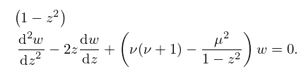
14.21.1 $$\left(1-z^2\right)\frac{d^{2}w}{{dz}^2}-2z\frac{dw}{dz}+\left(\nu (\nu +1)-\frac{{\mu }^2}{1-z^2}\right)w=0.$$

ⓘ

Symbols:

$\frac{df}{dx}$: derivative of $f$ with respect to $x$ , $z$: complex variable, $\mu$: general order and $\nu$: general degree

A&S Ref:

8.1.1

Referenced by:

§14.21(ii), §14.29, 2nd item

Permalink:

http://dlmf.nist.gov/14.21.E1

Encodings:

pMML, png, TeX

See also:

Annotations for §14.21(i), §14.21 and Ch.14

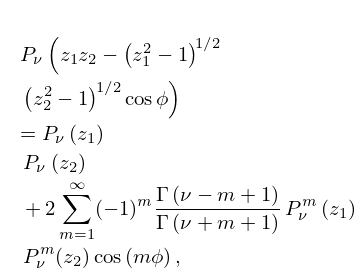
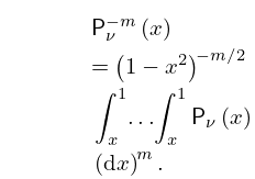
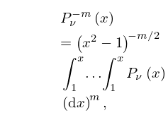
►Standard solutions: the associated Legendre functions $P_{\nu }^{\mu }\left(z\right)$, $P_{\nu }^{-\mu }\left(z\right)$, ${𝑸}_{\nu }^{\mu }\left(z\right)$, and ${𝑸}_{-\nu -1}^{\mu }\left(z\right)$. … … ►

§14.21(iii) Properties

… ►The generating function expansions (14.7.19) (with $𝖯$ replaced by $P$) and (14.7.22) apply when ; (14.7.21) (with $𝖯$ replaced by $P$) applies when $|h|>\max \left|z\pm {\left(z^2-1\right)}^{1/2}\right|$.

5: 14.26 Uniform Asymptotic Expansions

§14.26 Uniform Asymptotic Expansions

…

6: 14.28 Sums

§14.28 Sums

►

§14.28(i) Addition Theorem

… ►

14.28.1 $$P_{\nu }\left(z_1{z}_2-{\left(z_1^2-1\right)}^{1/2}{\left(z_2^2-1\right)}^{1/2}\cos \varphi \right)=P_{\nu }\left(z_1\right)P_{\nu }\left(z_2\right)+2\sum _{m=1}^{\mathrm{\infty }}{(-1)}^m\frac{\mathrm{\Gamma }\left(\nu -m+1\right)}{\mathrm{\Gamma }\left(\nu +m+1\right)}{P}_{\nu }^m\left(z_1\right)P_{\nu }^m(z_2)\cos \left(m\varphi \right),$$

ⓘ

Symbols:

$\mathrm{\Gamma }\left(z\right)$: gamma function, $P_{\nu }^{\mu }\left(z\right)$: associated Legendre function of the first kind, $\cos z$: cosine function, $P_{\nu }\left(z\right)=P_{\nu }^0\left(z\right)$: Legendre function of the first kind, $z$: complex variable, $m$: nonnegative integer and $\nu$: general degree

Permalink:

http://dlmf.nist.gov/14.28.E1

Encodings:

pMML, png, TeX

See also:

Annotations for §14.28(i), §14.28 and Ch.14

… ►

§14.28(ii) Heine’s Formula

►

14.28.2 $$\sum _{n=0}^{\mathrm{\infty }}(2n+1)Q_n\left(z_1\right)P_n\left(z_2\right)=\frac{1}{z_1-z_2},$$ $z_1\in {ℰ}_1$, $z_2\in {ℰ}_2$,

ⓘ

Symbols:

$\in$: element of, $P_{\nu }\left(z\right)=P_{\nu }^0\left(z\right)$: Legendre function of the first kind, $Q_{\nu }\left(z\right)=Q_{\nu }^0\left(z\right)$: Legendre function of the second kind, $z$: complex variable, $n$: nonnegative integer and ${ℰ}_1$, ${ℰ}_2$: ellipses

Permalink:

http://dlmf.nist.gov/14.28.E2

Encodings:

pMML, png, TeX

See also:

Annotations for §14.28(ii), §14.28 and Ch.14

…

7: 14.29 Generalizations

… ►are called Generalized Associated Legendre Functions. … …

8: 14.22 Graphics

§14.22 Graphics

… ►

►

►

Figure 14.22.4: ${𝑸}_0^0\left(x+\mathrm{i}y\right)$, $-5\le x\le 5$, $-5\le y\le 5$. … Magnify 3D Help

9: 14.6 Integer Order

§14.6 Integer Order

… ►

14.6.6 $${𝖯}_{\nu }^{-m}\left(x\right)={\left(1-x^2\right)}^{-m/2}{\int }_x^1\mathrm{\dots }{\int }_x^1{𝖯}_{\nu }\left(x\right){\left(dx\right)}^m.$$

ⓘ

Symbols:

: Ferrers function of the first kind, $dx$: differential of $x$ , $\int$: integral, ${𝖯}_{\nu }\left(x\right)={𝖯}_{\nu }^0\left(x\right)$: Ferrers function of the first kind, $P_{\nu }\left(z\right)=P_{\nu }^0\left(z\right)$: Legendre function of the first kind, $x$: real variable, $m$: nonnegative integer and $\nu$: general degree

Referenced by:

§14.12(i), Erratum (V1.0.28) for Equation (14.6.6)

Permalink:

http://dlmf.nist.gov/14.6.E6

Encodings:

pMML, png, TeX

Clarification (effective with 1.0.28):

The right-hand side has been corrected by replacing the Legendrefunction $P_{\nu }\left(x\right)$ with the Ferrers function ${𝖯}_{\nu }\left(x\right)$.

See also:

Annotations for §14.6(ii), §14.6 and Ch.14

►

14.6.7 $$P_{\nu }^{-m}\left(x\right)={\left(x^2-1\right)}^{-m/2}{\int }_1^x\mathrm{\dots }{\int }_1^x{P}_{\nu }\left(x\right){\left(dx\right)}^m,$$

ⓘ

Symbols:

$P_{\nu }^{\mu }\left(z\right)$: associated Legendre function of the first kind, $dx$: differential of $x$ , $\int$: integral, $P_{\nu }\left(z\right)=P_{\nu }^0\left(z\right)$: Legendre function of the first kind, $x$: real variable, $m$: nonnegative integer and $\nu$: general degree

A&S Ref:

8.14.17

Referenced by:

§14.21(iii)

Permalink:

http://dlmf.nist.gov/14.6.E7

Encodings:

pMML, png, TeX

See also:

Annotations for §14.6(ii), §14.6 and Ch.14

►

14.6.8 $$Q_{\nu }^{-m}\left(x\right)={(-1)}^m{\left(x^2-1\right)}^{-m/2}{\int }_x^{\mathrm{\infty }}\mathrm{\dots }{\int }_x^{\mathrm{\infty }}{Q}_{\nu }\left(x\right){\left(dx\right)}^m.$$

ⓘ

Symbols:

$Q_{\nu }^{\mu }\left(z\right)$: associated Legendre function of the second kind, $dx$: differential of $x$ , $\int$: integral, $Q_{\nu }\left(z\right)=Q_{\nu }^0\left(z\right)$: Legendre function of the second kind, $x$: real variable, $m$: nonnegative integer and $\nu$: general degree

A&S Ref:

8.14.18

Referenced by:

§14.21(iii)

Permalink:

http://dlmf.nist.gov/14.6.E8

Encodings:

pMML, png, TeX

See also:

Annotations for §14.6(ii), §14.6 and Ch.14

… ►

10: 14.27 Zeros

§14.27 Zeros

…