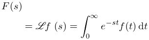
Laplace transforms

SearchAdvancedHelp

(0.003 seconds)

1—10 of 45 matching pages

1: 1.14 Integral Transforms

… ►

§1.14(iii) Laplace Transform

… ►

Inversion

… ►

Translation

… ►

Derivatives

… ►

1.14.31 $$ℒ\left(f\ast g\right)=ℒ\left(f\right)ℒ\left(g\right).$$

ⓘ

Symbols:

$ℒ\left(f\right)\left(s\right)$: Laplace transform and $\ast$: convolution (Laplace)

Keywords:

Laplacetransform

Permalink:

http://dlmf.nist.gov/1.14.E31

Encodings:

pMML, png, TeX

See also:

Annotations for §1.14(iii), §1.14(iii), §1.14 and Ch.1

…

2: 35.2 Laplace Transform

§35.2 Laplace Transform

►

Definition

… ►

Inversion Formula

… ►

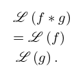
Convolution Theorem

►If $g_j$ is the Laplace transform of $f_j$, $j=1,2$, then $g_1{g}_2$ is the Laplace transform of the convolution $f_1\ast f_2$, where …

3: 16.20 Integrals and Series

… ►Extensive lists of Laplace transforms and inverse Laplace transforms of the Meijer $G$-function are given in Prudnikov et al. (1992a, §3.40) and Prudnikov et al. (1992b, §3.38). …

4: 19.13 Integrals of Elliptic Integrals

… ►

§19.13(iii) Laplace Transforms

►For direct and inverse Laplace transforms for the complete elliptic integrals $K\left(k\right)$, $E\left(k\right)$, and $D\left(k\right)$ see Prudnikov et al. (1992a, §3.31) and Prudnikov et al. (1992b, §§3.29 and 4.3.33), respectively.

5: 2.5 Mellin Transform Methods

… ►

§2.5(iii) Laplace Transforms with Small Parameters

… ►

2.5.37 $$ℒh\left(\zeta \right)={\int }_0^{\mathrm{\infty }}h(t){\mathrm{e}}^{-\zeta t}dt.$$

ⓘ

Symbols:

$ℒ\left(f\right)\left(s\right)$: Laplace transform, $dx$: differential of $x$ , $\mathrm{e}$: base of natural logarithm, $\int$: integral and $h(x)$: locally integrable function

Keywords:

Laplacetransform

Permalink:

http://dlmf.nist.gov/2.5.E37

Encodings:

pMML, png, TeX

Notational Change (effective with 1.0.15):

The notation for the Laplacetransform was changed to $ℒf\left(z\right)$ from $ℒ(f;z)$.

See also:

Annotations for §2.5(iii), §2.5 and Ch.2

… ►

2.5.38 $$\zeta ℒh\left(\zeta \right)=I_1(x)+I_2(x),$$

ⓘ

Symbols:

$ℒ\left(f\right)\left(s\right)$: Laplace transform, $h(x)$: locally integrable function and $I_j(x)$: integral

Keywords:

Laplacetransform

Referenced by:

§2.5(iii)

Permalink:

http://dlmf.nist.gov/2.5.E38

Encodings:

pMML, png, TeX

Notational Change (effective with 1.0.15):

The notation for the Laplacetransform was changed to $ℒf\left(z\right)$ from $ℒ(f;z)$.

See also:

Annotations for §2.5(iii), §2.5 and Ch.2

… ►

2.5.45 $$ℒh\left(\zeta \right)={\int }_0^{\mathrm{\infty }}\frac{{\mathrm{e}}^{-\zeta t}}{1+t}dt,$$ $\mathrm{\Re }\zeta >0$.

ⓘ

Symbols:

$ℒ\left(f\right)\left(s\right)$: Laplace transform, $dx$: differential of $x$ , $\mathrm{e}$: base of natural logarithm, $\int$: integral, $\mathrm{\Re }$: real part and $h(x)$: locally integrable function

Keywords:

Laplacetransform

Permalink:

http://dlmf.nist.gov/2.5.E45

Encodings:

pMML, png, TeX

Notational Change (effective with 1.0.15):

The notation for the Laplacetransform was changed to $ℒf\left(z\right)$ from $ℒ(f;z)$.

See also:

Annotations for §2.5(iii), §2.5(iii), §2.5 and Ch.2

… ►

2.5.49 $$ℒh\left(\zeta \right)={\mathrm{e}}^{\zeta }{E}_1\left(\zeta \right);$$

ⓘ

Symbols:

$ℒ\left(f\right)\left(s\right)$: Laplace transform, $\mathrm{e}$: base of natural logarithm, $E_1\left(z\right)$: exponential integral and $h(x)$: locally integrable function

Keywords:

Laplacetransform

Permalink:

http://dlmf.nist.gov/2.5.E49

Encodings:

pMML, png, TeX

Notational Change (effective with 1.0.15):

The notation for the Laplacetransform was changed to $ℒf\left(z\right)$ from $ℒ(f;z)$.

See also:

Annotations for §2.5(iii), §2.5(iii), §2.5 and Ch.2

…

6: 15.14 Integrals

… ►Laplace transforms of hypergeometric functions are given in Erdélyi et al. (1954a, §4.21), Oberhettinger and Badii (1973, §1.19), and Prudnikov et al. (1992a, §3.37). Inverse Laplace transforms of hypergeometric functions are given in Erdélyi et al. (1954a, §5.19), Oberhettinger and Badii (1973, §2.18), and Prudnikov et al. (1992b, §3.35). …

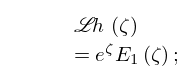
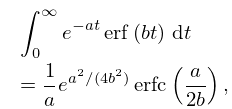
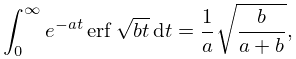
7: 6.14 Integrals

… ►

§6.14(i) Laplace Transforms

…

8: 7.14 Integrals

… ►

Laplace Transforms

►

7.14.2 $${\int }_0^{\mathrm{\infty }}{\mathrm{e}}^{-at}\mathrm{erf}\left(bt\right)dt=\frac{1}{a}{\mathrm{e}}^{a^2/(4b^2)}\mathrm{erfc}\left(\frac{a}{2b}\right),$$ $\mathrm{\Re }a>0$, ,

ⓘ

Symbols:

$\pi$: the ratio of the circumference of a circle to its diameter, $\mathrm{erfc}z$: complementary error function, $dx$: differential of $x$ , $\mathrm{erf}z$: error function, $\mathrm{e}$: base of natural logarithm, $\int$: integral, $\mathrm{ph}$: phase and $\mathrm{\Re }$: real part

Keywords:

Laplacetransform

A&S Ref:

7.4.17

Referenced by:

§7.14(i)

Permalink:

http://dlmf.nist.gov/7.14.E2

Encodings:

pMML, png, TeX

See also:

Annotations for §7.14(i), §7.14(i), §7.14 and Ch.7

►

7.14.3 $${\int }_0^{\mathrm{\infty }}{\mathrm{e}}^{-at}\mathrm{erf}\sqrt{bt}dt=\frac{1}{a}\sqrt{\frac{b}{a+b}},$$ $\mathrm{\Re }a>0$, $\mathrm{\Re }b>0$,

ⓘ

Symbols:

$dx$: differential of $x$ , $\mathrm{erf}z$: error function, $\mathrm{e}$: base of natural logarithm, $\int$: integral and $\mathrm{\Re }$: real part

Keywords:

Laplacetransform

A&S Ref:

7.4.19

Referenced by:

§7.14(i)

Permalink:

http://dlmf.nist.gov/7.14.E3

Encodings:

pMML, png, TeX

See also:

Annotations for §7.14(i), §7.14(i), §7.14 and Ch.7

►

7.14.4 $${\int }_0^{\mathrm{\infty }}{\mathrm{e}}^{(a-b)t}\mathrm{erfc}\left(\sqrt{at}+\sqrt{\frac{c}{t}}\right)dt=\frac{{\mathrm{e}}^{-2(\sqrt{ac}+\sqrt{bc})}}{\sqrt{b}(\sqrt{a}+\sqrt{b})},$$ , $\mathrm{\Re }b>0$, $\mathrm{\Re }c\ge 0$.

ⓘ

Symbols:

$\pi$: the ratio of the circumference of a circle to its diameter, $\mathrm{erfc}z$: complementary error function, $dx$: differential of $x$ , $\mathrm{e}$: base of natural logarithm, $\int$: integral, $\mathrm{ph}$: phase and $\mathrm{\Re }$: real part

Keywords:

Laplacetransform

A&S Ref:

7.4.21

Referenced by:

§3.5(ix), §7.14(i)

Permalink:

http://dlmf.nist.gov/7.14.E4

Encodings:

pMML, png, TeX

See also:

Annotations for §7.14(i), §7.14(i), §7.14 and Ch.7

… ►

Laplace Transforms

…

9: 3.11 Approximation Techniques

… ►

Laplace Transform Inversion

►Numerical inversion of the Laplace transform (§1.14(iii)) ►

3.11.26 $$F(s)=ℒf\left(s\right)={\int }_0^{\mathrm{\infty }}{\mathrm{e}}^{-st}f(t)dt$$

ⓘ

Defines:

$F(s)$: Laplace transform of $f(t)$ (locally)

Symbols:

$ℒ\left(f\right)\left(s\right)$: Laplace transform, $dx$: differential of $x$ , $\mathrm{e}$: base of natural logarithm and $\int$: integral

Keywords:

Laplacetransform

A&S Ref:

29.1.1

Permalink:

http://dlmf.nist.gov/3.11.E26

Encodings:

pMML, png, TeX

Notational Change (effective with 1.0.15):

The notation for the Laplacetransform was changed to $ℒf\left(z\right)$ from $ℒ(f;z)$.

See also:

Annotations for §3.11(iv), §3.11(iv), §3.11 and Ch.3

►requires $f={ℒ}^{-1}F$ to be obtained from numerical values of $F$. A general procedure is to approximate $F$ by a rational function $R$ (vanishing at infinity) and then approximate $f$ by $r={ℒ}^{-1}R$. …

10: 2.4 Contour Integrals

… ►Then … ►For examples and extensions (including uniformity and loop integrals) see Olver (1997b, Chapter 4), Wong (1989, Chapter 1), and Temme (1985). ►

§2.4(ii) Inverse Laplace Transforms

… ►Then the Laplace transform … ►For examples see Olver (1997b, pp. 315–320). …