Laplace equation

SearchAdvancedHelp

(0.001 seconds)

11—20 of 36 matching pages

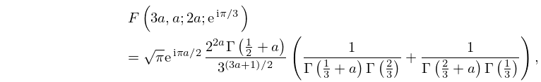
11: 15.4 Special Cases

… ►

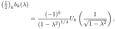
15.4.34 $$F(3a,a;2a;{\mathrm{e}}^{\mathrm{i}\pi /3})=\sqrt{\pi }{\mathrm{e}}^{\mathrm{i}\pi a/2}\frac{2^{2a}\mathrm{\Gamma }\left(\frac{1}{2}+a\right)}{3^{(3a+1)/2}}\left(\frac{1}{\mathrm{\Gamma }\left(\frac{1}{3}+a\right)\mathrm{\Gamma }\left(\frac{2}{3}\right)}+\frac{1}{\mathrm{\Gamma }\left(\frac{2}{3}+a\right)\mathrm{\Gamma }\left(\frac{1}{3}\right)}\right),$$

ⓘ

Symbols:

$\mathrm{\Gamma }\left(z\right)$: gamma function, $F(a,b;c;z)$ or $F(\genfrac{}{}{0pt}{}{a,b}{c};z)$: $={}_2{}^{}F_1^{}(a,b;c;z)$ Gauss’ hypergeometric function, $\pi$: the ratio of the circumference of a circle to its diameter, $\mathrm{e}$: base of natural logarithm, $\mathrm{i}$: imaginary unit and $a$: real or complex parameter

Proof sketch:

From §15.5(ii) one obtains that $w(a)={\mathrm{e}}^{-\mathrm{i}\pi a/2}{2}^{-2a}{3}^{(3a+1)/2}F(3a,a;2a;{\mathrm{e}}^{\mathrm{i}\pi /3})\mathrm{\Gamma }\left(\frac{1}{3}+a\right)/\mathrm{\Gamma }\left(\frac{1}{2}+a\right)$ is a solution of the difference equation $(3a+5)w(a+2)-6(a+1)w(a+1)+(3a+1)w(a)=0$. Two linearly independent solutions of this difference equation are $w_1(a)=1$ and $w_2(a)=\mathrm{\Gamma }\left(\frac{1}{3}+a\right)/\mathrm{\Gamma }\left(\frac{2}{3}+a\right)$. Combining (15.6.1) with Laplace’s method (see §2.4(iii)) we obtain that $w(a)\sim \sqrt{\pi }\left(\frac{1}{\mathrm{\Gamma }\left(\frac{2}{3}\right)}+\frac{a^{-1/3}}{\mathrm{\Gamma }\left(\frac{1}{3}\right)}\right)$, as $a\to \mathrm{\infty }$. Hence, $w(a)=\sqrt{\pi }\left(\frac{1}{\mathrm{\Gamma }\left(\frac{2}{3}\right)}+\frac{w_2(a)}{\mathrm{\Gamma }\left(\frac{1}{3}\right)}\right)$.

Notes:

See §15.2(ii) for treatment of the case when the third parameter is a nonpositive integer.

Referenced by:

§15.4(iii), §15.4(iii), Erratum (V1.1.2) for Additions

Permalink:

http://dlmf.nist.gov/15.4.E34

Encodings:

pMML, png, TeX

Addition (effective with 1.1.2):

This equation was added.

See also:

Annotations for §15.4(iii), §15.4 and Ch.15

…

12: 35.7 Gaussian Hypergeometric Function of Matrix Argument

… ►

§35.7(iii) Partial Differential Equations

… ►Subject to the conditions (a)–(c), the function $f(𝐓)={}_2{}^{}F_1^{}(a,b;c;𝐓)$ is the unique solution of each partial differential equation … ►Systems of partial differential equations for the ${}_0{}^{}F_1^{}$ (defined in §35.8) and ${}_1{}^{}F_1^{}$ functions of matrix argument can be obtained by applying (35.8.9) and (35.8.10) to (35.7.9). … ►Butler and Wood (2002) applies Laplace’s method (§2.3(iii)) to (35.7.5) to derive uniform asymptotic approximations for the functions …

13: Bibliography K

… ►

Asymptotic behavior of the solutions of the Painlevé equation of the first kind. Differ. Uravn. 24 (10), pp. 1684–1695 (Russian).

ⓘ

Notes:

In Russian. English translation: Differential Equations 24(1988), no. 10, pp. 1107–1115 (1989)

External Links:

ISSN 0374-0641, MathReview, ZentralBlatt

Referenced by:

§32.11(i).

Encodings:

BibTeX

… ►

Rational solutions of the fifth Painlevé equation. Differential Integral Equations 7 (3-4), pp. 967–1000.

ⓘ

External Links:

ISSN 0893-4983, MathReview, ZentralBlatt

Referenced by:

§32.8(v).

Encodings:

BibTeX

… ►

Asymptotic solution of Maxwell’s equations near caustics. Izv. Vuz. Radiofiz. 7, pp. 1049–1056.

ⓘ

Referenced by:

§36.14(i).

Encodings:

BibTeX

… ►

The Korteweg-de Vries Equation and Related Evolution Equations. In Nonlinear Wave Motion (Proc. AMS-SIAM Summer Sem., Clarkson Coll. Tech., Potsdam, N.Y., 1972), A. C. Newell (Ed.), Lectures in Appl. Math., Vol. 15, pp. 61–83.

ⓘ

External Links:

MathReview (G. L. Lamb, Jr.), ZentralBlatt

Referenced by:

§22.19(iii).

Encodings:

BibTeX

►

A Handbook of Methods of Approximate Fourier Transformation and Inversion of the Laplace Transformation. Mir, Moscow.

ⓘ

Notes:

Translated from the Russian by George Yankovsky. Reprint of the 1977 translation

External Links:

MathReview, ZentralBlatt

Referenced by:

§3.5(viii).

Encodings:

BibTeX

…

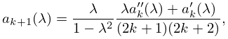
14: 3.11 Approximation Techniques

… ►Also, in cases where $f(x)$ satisfies a linear ordinary differential equation with polynomial coefficients, the expansion (3.11.11) can be substituted in the differential equation to yield a recurrence relation satisfied by the $c_n$. … ►

Laplace Transform Inversion

►Numerical inversion of the Laplace transform (§1.14(iii)) …requires $f={ℒ}^{-1}F$ to be obtained from numerical values of $F$. A general procedure is to approximate $F$ by a rational function $R$ (vanishing at infinity) and then approximate $f$ by $r={ℒ}^{-1}R$. …

15: Bibliography L

… ►

Some differential equations and associated integral equations. Quart. J. Math. (Oxford) 5, pp. 81–97.

ⓘ

External Links:

Document, ZentralBlatt

Referenced by:

§31.10(i), §31.9(i).

Encodings:

BibTeX

… ►

Solutions to a generalized spheroidal wave equation: Teukolsky’s equations in general relativity, and the two-center problem in molecular quantum mechanics. J. Math. Phys. 27 (5), pp. 1238–1265.

ⓘ

External Links:

ISSN 0022-2488, Document, MathReview (Basilis C. Xanthopoulos), ZentralBlatt

Referenced by:

§30.12, §31.17(ii).

Encodings:

BibTeX

… ►

Error bounds for asymptotic expansions of Laplace convolutions. SIAM J. Math. Anal. 25 (6), pp. 1537–1553.

ⓘ

External Links:

ISSN 0036-1410, Document, MathReview (Walter Schempp), ZentralBlatt

Referenced by:

§2.6(iii).

Encodings:

BibTeX

… ►

Well-posedness and blow-up solutions for an integrable nonlinearly dispersive model wave equation. J. Differential Equations 162 (1), pp. 27–63.

ⓘ

External Links:

ISSN 0022-0396, Document, MathReview (John Albert), ZentralBlatt

Referenced by:

§22.19(iii).

Encodings:

BibTeX

… ►

The second Painlevé equation. Differ. Uravn. 7 (6), pp. 1124–1125 (Russian).

ⓘ

Notes:

In Russian. English translation: Differential Equations 7(6), pp. 853–854

External Links:

MathReview (Z. Rubinstein), ZentralBlatt

Referenced by:

§32.7(ii).

Encodings:

BibTeX

…

16: Frank W. J. Olver

… ►He is particularly known for his extensive work in the study of the asymptotic solution of differential equations, i. …, the behavior of solutions as the independent variable, or some parameter, tends to infinity, and in the study of the particular solutions of differential equations known as special functions (e. … ►In a review of that volume, Jet Wimp of Drexel University said that the papers “exemplify a redoubtable mathematical talent, the work of a man who has done more than almost anyone else in the 20th century to bestow on the discipline of applied mathematics the elegance and rigor that its earliest practitioners, such as Gauss and Laplace, would have wished for it. …

17: Bibliography N

… ►

Toda equation and its solutions in special functions. J. Phys. Soc. Japan 65 (6), pp. 1589–1597.

ⓘ

External Links:

ISSN 0031-9015, Document, MathReview, ZentralBlatt

Referenced by:

§18.38(ii).

Encodings:

BibTeX

… ►

Confluent hypergeometric equations and related solvable potentials in quantum mechanics. J. Math. Phys. 41 (12), pp. 7964–7996.

ⓘ

External Links:

ISSN 0022-2488, Document, MathReview, ZentralBlatt

Referenced by:

§13.28(i).

Encodings:

BibTeX

… ►

An explicit formula for the coefficients in Laplace’s method. Constr. Approx. 38 (3), pp. 471–487.

ⓘ

External Links:

ISSN 0176-4276, Document, Link, MathReview (Pedro J. Pagola), ZentralBlatt

Referenced by:

§5.11(i), §5.11(i).

Encodings:

BibTeX

… ►

An extension of Laplace’s method. Constr. Approx. 51 (2), pp. 247–272.

ⓘ

External Links:

ISSN 0176-4276, Document, Link, MathReview (José Luis López), ZentralBlatt

Referenced by:

(11.11.16), (11.11.17), §11.11(iii).

Encodings:

BibTeX

… ►

Solving equations exactly. J. Res. Nat. Bur. Standards Sect. B 71B, pp. 171–179.

ⓘ

External Links:

MathReview, ZentralBlatt

Referenced by:

§27.15.

Encodings:

BibTeX

…

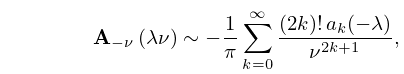
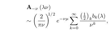
18: 11.11 Asymptotic Expansions of Anger–Weber Functions

… ►

11.11.9_5 $$a_{k+1}(\lambda )=\frac{\lambda }{1-{\lambda }^2}\frac{\lambda a_k^{\prime \prime }(\lambda )+a_k^{\prime }(\lambda )}{(2k+1)(2k+2)},$$ $k=0,1,2,\mathrm{\dots }$.

ⓘ

Symbols:

$k$: nonnegative integer, $\lambda$: parameter and $a_k(\lambda )$: expansion function

Referenced by:

Erratum (V1.1.2) for Additions

Permalink:

http://dlmf.nist.gov/11.11.E9_5

Encodings:

pMML, png, TeX

Addition (effective with 1.1.2):

This equation was added.

See also:

Annotations for §11.11(iii), §11.11 and Ch.11

… ►

11.11.10 $${𝐀}_{-\nu }\left(\lambda \nu \right)\sim -\frac{1}{\pi }\sum _{k=0}^{\mathrm{\infty }}\frac{(2k)!a_k(-\lambda )}{{\nu }^{2k+1}},$$ $\nu \to \mathrm{\infty }$, $|\mathrm{ph}\nu |\le \pi -\delta$.

ⓘ

Symbols:

${𝐀}_{\nu }\left(z\right)$: Anger–Weber function, $\sim$: Poincaré asymptotic expansion, $\pi$: the ratio of the circumference of a circle to its diameter, $!$: factorial (as in $n!$), $\mathrm{ph}$: phase, $\nu$: real or complex order, $k$: nonnegative integer, $\delta$: arbitrary small positive constant, $\lambda$: parameter and $a_k(\lambda )$: expansion function

Sources:

Meijer (1932); Watson (1944, §10.15); Olver (1997b, pp. 103 and 352); Nemes (2014b); Nemes (2014c)

Proof sketch:

Apply Laplace’s method to the integral (11.10.4).

Referenced by:

(11.11.18), (11.11.19), §11.11(iii), §11.11(iii)

Permalink:

http://dlmf.nist.gov/11.11.E10

Encodings:

pMML, png, TeX

Clarification (effective with 1.1.2):

The constraint which was originally $\nu \to +\mathrm{\infty }$, has been extended to be $\nu \to \mathrm{\infty }$, $|\mathrm{ph}\nu |\le \pi -\delta$.

Suggested 2021-04-05 by Gergő Nemes

See also:

Annotations for §11.11(iii), §11.11 and Ch.11

… ►

11.11.11 $${𝐀}_{-\nu }\left(\lambda \nu \right)\sim {\left(\frac{2}{\pi \nu }\right)}^{1/2}{\mathrm{e}}^{-\nu \mu }\sum _{k=0}^{\mathrm{\infty }}\frac{{\left(\frac{1}{2}\right)}_k{b}_k(\lambda )}{{\nu }^k},$$ $\nu \to \mathrm{\infty }$, $|\mathrm{ph}\nu |\le \frac{\pi }{2}-\delta$,

ⓘ

Symbols:

${\left(a\right)}_n$: Pochhammer’s symbol (or shifted factorial), ${𝐀}_{\nu }\left(z\right)$: Anger–Weber function, $\sim$: Poincaré asymptotic expansion, $\pi$: the ratio of the circumference of a circle to its diameter, $\mathrm{e}$: base of natural logarithm, $\mathrm{ph}$: phase, $\nu$: real or complex order, $k$: nonnegative integer, $\delta$: arbitrary small positive constant, $\lambda$: parameter and $b_k(\lambda )$: expansion function

Sources:

Dingle (1973, p. 388); Olver (1997b, pp. 103 and 352)

Proof sketch:

Derivable by applying Laplace’s method to the integral (11.10.4).

Permalink:

http://dlmf.nist.gov/11.11.E11

Encodings:

pMML, png, TeX

Clarification (effective with 1.1.2):

The constraint which was originally $\nu \to +\mathrm{\infty }$, has been extended to be $\nu \to \mathrm{\infty }$, $|\mathrm{ph}\nu |\le \frac{\pi }{2}-\delta$.

Suggested 2021-04-05 by Gergő Nemes

See also:

Annotations for §11.11(iii), §11.11 and Ch.11

… ►

11.11.13_5 $${\left(\frac{1}{2}\right)}_k{b}_k(\lambda )=\frac{{(-1)}^k}{{\left(1-{\lambda }^2\right)}^{1/4}}{U}_k\left(\frac{1}{\sqrt{1-{\lambda }^2}}\right),$$ $k=0,1,2,\mathrm{\dots }$,

ⓘ

Symbols:

${\left(a\right)}_n$: Pochhammer’s symbol (or shifted factorial), $k$: nonnegative integer, $\lambda$: parameter and $b_k(\lambda )$: expansion function

Referenced by:

Erratum (V1.1.2) for Additions

Permalink:

http://dlmf.nist.gov/11.11.E13_5

Encodings:

pMML, png, TeX

Addition (effective with 1.1.2):

This equation was added.

See also:

Annotations for §11.11(iii), §11.11 and Ch.11

…

19: Bibliography S

… ►

Orthogonal polynomials arising in the numerical evaluation of inverse Laplace transforms. Math. Tables Aids Comput. 9 (52), pp. 164–177.

ⓘ

External Links:

FullText, MathReview (S. C. van Veen), ZentralBlatt

Referenced by:

§3.5(viii).

Encodings:

BibTeX

… ►

The Laplace Transform: Theory and Applications. Undergraduate Texts in Mathematics, Springer-Verlag, New York.

ⓘ

External Links:

ISBN 0-387-98698-7, MathReview (Philip Heywood), ZentralBlatt

Referenced by:

§1.14(iii), §1.14(vii).

Encodings:

BibTeX

… ►

The Laplace transforms of products of Airy functions. Dirāsāt Ser. B Pure Appl. Sci. 19 (2), pp. 7–11.

ⓘ

External Links:

ISSN 0253-424X, MathReview

Referenced by:

§9.10(v).

Encodings:

BibTeX

… ►

Characterization of Jacobian varieties in terms of soliton equations. Invent. Math. 83 (2), pp. 333–382.

ⓘ

External Links:

ISSN 0020-9910, Document, MathReview (Bert van Geemen), ZentralBlatt

Referenced by:

§21.9.

Encodings:

BibTeX

… ►

The linear differential equation whose solutions are the products of solutions of two given differential equations. J. Math. Anal. Appl. 98 (1), pp. 130–147.

ⓘ

External Links:

ISSN 0022-247X, Document, FullText, MathReview (Wolfgang Bühring), ZentralBlatt

Referenced by:

§1.13(v).

Encodings:

BibTeX

…

20: 3.5 Quadrature

… ►

Example. Laplace Transform Inversion

… ►Equation (3.5.36), without the error term, becomes … ►

Table 3.5.19: Laplace transform inversion.

► ►►

$t$	$J_0(t)$	$g(t)$
…

►

… ►In fact from (7.14.4) and the inversion formula for the Laplace transform (§1.14(iii)) we have … ►A special case is the rule for Hilbert transforms (§1.14(v)): …