Laguerre functions

SearchAdvancedHelp

(0.005 seconds)

1—10 of 47 matching pages

1: 35.6 Confluent Hypergeometric Functions of Matrix Argument

… ►

Laguerre Form

►

35.6.3 $$L_{\nu }^{(\gamma )}\left(𝐓\right)=\frac{{\mathrm{\Gamma }}_m\left(\gamma +\nu +\frac{1}{2}(m+1)\right)}{{\mathrm{\Gamma }}_m\left(\gamma +\frac{1}{2}(m+1)\right)}{}_1{}^{}F_1^{}(\genfrac{}{}{0pt}{}{-\nu }{\gamma +\frac{1}{2}(m+1)};𝐓),$$ $\mathrm{\Re }\left(\gamma \right),\mathrm{\Re }\left(\gamma +\nu \right)>-1$.

ⓘ

Defines:

$L_{\nu }^{(\gamma )}\left(𝐓\right)$: Laguerre function of matrix argument

Symbols:

${}_p{}^{}F_q^{}(a_1,\mathrm{\dots },a_p;b_1,\mathrm{\dots },b_q;𝐓)$ or ${}_p{}^{}F_q^{}(\genfrac{}{}{0pt}{}{a_1,\mathrm{\dots },a_p}{b_1,\mathrm{\dots },b_q};𝐓)$: generalized hypergeometric function of matrix argument, ${\mathrm{\Gamma }}_m\left(a\right)$: multivariate gamma function, $\mathrm{\Re }$: real part, $𝐓$: real symmetric $m\times m$ matrix and $m$: positive integer

Permalink:

http://dlmf.nist.gov/35.6.E3

Encodings:

pMML, png, TeX

See also:

Annotations for §35.6(i), §35.6(i), §35.6 and Ch.35

…

2: 33.22 Particle Scattering and Atomic and Molecular Spectra

… ►The functions ${\varphi }_{n,\mathrm{\ell }}(r)$ defined by (33.14.14) are the hydrogenic bound states in attractive Coulomb potentials; their polynomial components are often called associated Laguerre functions; see Christy and Duck (1961) and Bethe and Salpeter (1977). …

3: 17.17 Physical Applications

… ►See Kassel (1995). …

4: Bibliography Y

… ►

Generalized Hypergeometric Functions and Laguerre Polynomials in Two Variables. In Hypergeometric Functions on Domains of Positivity, Jack Polynomials, and Applications (Tampa, FL, 1991), Contemporary Mathematics, Vol. 138, pp. 239–259.

ⓘ

External Links:

MathReview (B. M. Agrawal), ZentralBlatt

Referenced by:

§35.10.

Encodings:

BibTeX

…

5: 18.34 Bessel Polynomials

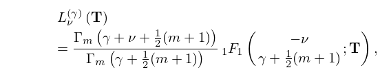
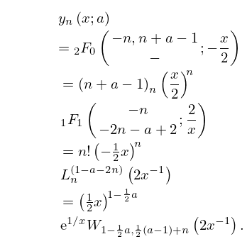
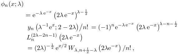
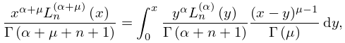
… ►For the confluent hypergeometric function ${}_1{}^{}F_1^{}$ and the generalized hypergeometric function ${}_2{}^{}F_0^{}$, the Laguerre polynomial $L_n^{(\alpha )}$ and the Whittaker function $W_{\kappa ,\mu }$ see §16.2(ii), §16.2(iv), (18.5.12), and (13.14.3), respectively. ►

18.34.1 $$y_n(x;a)={}_2{}^{}F_0^{}(\genfrac{}{}{0pt}{}{-n,n+a-1}{-};-\frac{x}{2})={\left(n+a-1\right)}_n{\left(\frac{x}{2}\right)}^n{}_1{}^{}F_1^{}(\genfrac{}{}{0pt}{}{-n}{-2n-a+2};\frac{2}{x})=n!{\left(-\frac{1}{2}x\right)}^n{L}_n^{(1-a-2n)}\left(2x^{-1}\right)={\left(\frac{1}{2}x\right)}^{1-\frac{1}{2}a}{\mathrm{e}}^{1/x}{W}_{1-\frac{1}{2}a,\frac{1}{2}(a-1)+n}\left(2x^{-1}\right).$$

ⓘ

Defines:

$y_n(x;a)$: Bessel polynomial

Symbols:

${}_p{}^{}F_q^{}(a_1,\mathrm{\dots },a_p;b_1,\mathrm{\dots },b_q;z)$ or ${}_p{}^{}F_q^{}(\genfrac{}{}{0pt}{}{a_1,\mathrm{\dots },a_p}{b_1,\mathrm{\dots },b_q};z)$: alternatively ${}_p{}^{}F_q^{}(𝐚;𝐛;z)$ or ${}_p{}^{}F_q^{}(\genfrac{}{}{0pt}{}{𝐚}{𝐛};z)$
generalized hypergeometric function, ${}_1{}^{}F_1^{}(a;b;z)$: $=M(a,b,z)$ notation for the Kummer confluent hypergeometric function, $L_n^{(\alpha )}\left(x\right)$: Laguerre (or generalized Laguerre) polynomial, ${\left(a\right)}_n$: Pochhammer’s symbol (or shifted factorial), $W_{\kappa ,\mu }\left(z\right)$: Whittaker confluent hypergeometric function, $\mathrm{e}$: base of natural logarithm, $!$: factorial (as in $n!$), $n$: nonnegative integer and $x$: real variable

Proved:

Grosswald (1978, p.38, Theorem 1); Combine (18.5.12) and items (i), (v), (vii) of the mentioned theorem for $b=2$(proved)

Referenced by:

(18.34.2), (18.34.7_1), §18.34(i), §18.34(i), Erratum (V1.2.0) for Equation (18.34.1)

Permalink:

http://dlmf.nist.gov/18.34.E1

Encodings:

pMML, png, TeX

Addition (effective with 1.2.0):

This equation was updated to include the definition of Bessel polynomials in terms of Laguerre polynomials and the Whittaker confluent hypergeometric function.

See also:

Annotations for §18.34(i), §18.34 and Ch.18

… ►

18.34.7_1 $${\varphi }_n(x;\lambda )={\mathrm{e}}^{-\lambda {\mathrm{e}}^{-x}}{\left(2\lambda {\mathrm{e}}^{-x}\right)}^{\lambda -\frac{1}{2}}{y}_n({\lambda }^{-1}{\mathrm{e}}^x;2-2\lambda )/n!={(-1)}^n{\mathrm{e}}^{-\lambda {\mathrm{e}}^{-x}}{\left(2\lambda {\mathrm{e}}^{-x}\right)}^{\lambda -n-\frac{1}{2}}{L}_n^{(2\lambda -2n-1)}\left(2\lambda {\mathrm{e}}^{-x}\right)={(2\lambda )}^{-\frac{1}{2}}{\mathrm{e}}^{x/2}{W}_{\lambda ,n+\frac{1}{2}-\lambda }\left(2\lambda {\mathrm{e}}^{-x}\right)/n!,$$ $n=0,1,\mathrm{\dots },N=\lceil \lambda -\frac{3}{2}\rceil$, $\lambda >\frac{1}{2}$,

ⓘ

Symbols:

$y_n(x;a)$: Bessel polynomial, $L_n^{(\alpha )}\left(x\right)$: Laguerre (or generalized Laguerre) polynomial, $W_{\kappa ,\mu }\left(z\right)$: Whittaker confluent hypergeometric function, $\lceil x\rceil$: ceiling of $x$ , $\mathrm{e}$: base of natural logarithm, $!$: factorial (as in $n!$), $N$: positive integer, $n$: nonnegative integer and $x$: real variable

Proof sketch:

The second and third equality follow from (18.34.1).

Referenced by:

(18.34.7_2), (18.34.7_3), §18.34(iii), (18.39.17), (18.39.18), §18.39(i), Erratum (V1.2.0) Section 18.34

Permalink:

http://dlmf.nist.gov/18.34.E7_1

Encodings:

pMML, png, TeX

Addition (effective with 1.2.0):

This equation was added.

See also:

Annotations for §18.34(iii), §18.34 and Ch.18

►expressed in terms of Romanovski–Bessel polynomials, Laguerre polynomials or Whittaker functions, we have …

6: 18.3 Definitions

… ►

Table 18.3.1: Orthogonality properties for classical OP’s: intervals, weight functions, standardizations, leading coefficients, and parameter constraints. …

► ►►

Name	$p_n(x)$	$(a,b)$	$w(x)$	$h_n$	$k_n$	${\tilde{k}}_n/k_n$	Constraints
…

►

…

7: 18.17 Integrals

… ►

18.17.14 $$\frac{x^{\alpha +\mu }{L}_n^{(\alpha +\mu )}\left(x\right)}{\mathrm{\Gamma }\left(\alpha +\mu +n+1\right)}={\int }_0^x\frac{y^{\alpha }{L}_n^{(\alpha )}\left(y\right)}{\mathrm{\Gamma }\left(\alpha +n+1\right)}\frac{{(x-y)}^{\mu -1}}{\mathrm{\Gamma }\left(\mu \right)}dy,$$ $\mu >0$, $x>0$.

ⓘ

Symbols:

$\mathrm{\Gamma }\left(z\right)$: gamma function, $L_n^{(\alpha )}\left(x\right)$: Laguerre (or generalized Laguerre) polynomial, $dx$: differential of $x$ , $\int$: integral, $y$: real variable, $n$: nonnegative integer and $x$: real variable

A&S Ref:

22.13.13

Referenced by:

§18.17(iv)

Permalink:

http://dlmf.nist.gov/18.17.E14

Encodings:

pMML, png, TeX

See also:

Annotations for §18.17(iv), §18.17(iv), §18.17 and Ch.18

►

18.17.15 $${\mathrm{e}}^{-x}{L}_n^{(\alpha )}\left(x\right)={\int }_x^{\mathrm{\infty }}{\mathrm{e}}^{-y}{L}_n^{(\alpha +\mu )}\left(y\right)\frac{{(y-x)}^{\mu -1}}{\mathrm{\Gamma }\left(\mu \right)}dy,$$ $\mu >0$.

ⓘ

Symbols:

$\mathrm{\Gamma }\left(z\right)$: gamma function, $L_n^{(\alpha )}\left(x\right)$: Laguerre (or generalized Laguerre) polynomial, $dx$: differential of $x$ , $\mathrm{e}$: base of natural logarithm, $\int$: integral, $y$: real variable, $n$: nonnegative integer and $x$: real variable

Referenced by:

§18.17(iv), §18.17(iv)

Permalink:

http://dlmf.nist.gov/18.17.E15

Encodings:

pMML, png, TeX

See also:

Annotations for §18.17(iv), §18.17(iv), §18.17 and Ch.18

… ►

18.17.28_5 $${\int }_0^{\mathrm{\infty }}{\mathrm{e}}^{-x}{x}^{\alpha }{L}_n^{(\alpha )}\left(x\right){\mathrm{e}}^{\mathrm{i}xy}dx=\frac{\mathrm{\Gamma }\left(\alpha +n+1\right){(-\mathrm{i}y)}^n}{n!{\left(1-\mathrm{i}y\right)}^{\alpha +n+1}},$$

ⓘ

Symbols:

$\mathrm{\Gamma }\left(z\right)$: gamma function, $L_n^{(\alpha )}\left(x\right)$: Laguerre (or generalized Laguerre) polynomial, $dx$: differential of $x$ , $\mathrm{e}$: base of natural logarithm, $!$: factorial (as in $n!$), $\mathrm{i}$: imaginary unit, $\int$: integral, $y$: real variable, $n$: nonnegative integer and $x$: real variable

Referenced by:

§18.17(v), Erratum (V1.2.0) Section 18.17

Permalink:

http://dlmf.nist.gov/18.17.E28_5

Encodings:

pMML, png, TeX

See also:

Annotations for §18.17(v), §18.17(v), §18.17 and Ch.18

… ►

18.17.31 $${\int }_0^{\mathrm{\infty }}{\mathrm{e}}^{-ax}{x}^{\nu -2n}{L}_{2n-1}^{(\nu -2n)}\left(ax\right)\cos \left(xy\right)dx=i\frac{{(-1)}^n\mathrm{\Gamma }\left(\nu \right)}{2(2n-1)!}{y}^{2n-1}\left({(a+iy)}^{-\nu }-{(a-iy)}^{-\nu }\right),$$ $\nu >2n-1$, $a>0$,

ⓘ

Symbols:

$\mathrm{\Gamma }\left(z\right)$: gamma function, $L_n^{(\alpha )}\left(x\right)$: Laguerre (or generalized Laguerre) polynomial, $\cos z$: cosine function, $dx$: differential of $x$ , $\mathrm{e}$: base of natural logarithm, $!$: factorial (as in $n!$), $\int$: integral, $y$: real variable, $n$: nonnegative integer and $x$: real variable

Referenced by:

§18.17(v)

Permalink:

http://dlmf.nist.gov/18.17.E31

Encodings:

pMML, png, TeX

See also:

Annotations for §18.17(v), §18.17(v), §18.17 and Ch.18

►

18.17.32 $${\int }_0^{\mathrm{\infty }}{\mathrm{e}}^{-ax}{x}^{\nu -1-2n}{L}_{2n}^{(\nu -1-2n)}\left(ax\right)\cos \left(xy\right)dx=\frac{{(-1)}^n\mathrm{\Gamma }\left(\nu \right)}{2(2n)!}{y}^{2n}\left({(a+iy)}^{-\nu }+{(a-iy)}^{-\nu }\right),$$ $\nu >2n$, $a>0$.

ⓘ

Symbols:

$\mathrm{\Gamma }\left(z\right)$: gamma function, $L_n^{(\alpha )}\left(x\right)$: Laguerre (or generalized Laguerre) polynomial, $\cos z$: cosine function, $dx$: differential of $x$ , $\mathrm{e}$: base of natural logarithm, $!$: factorial (as in $n!$), $\int$: integral, $y$: real variable, $n$: nonnegative integer and $x$: real variable

Referenced by:

§18.17(v)

Permalink:

http://dlmf.nist.gov/18.17.E32

Encodings:

pMML, png, TeX

See also:

Annotations for §18.17(v), §18.17(v), §18.17 and Ch.18

…

8: 18.11 Relations to Other Functions

… ►

Laguerre

►

18.11.2 $$L_n^{(\alpha )}\left(x\right)=\frac{{\left(\alpha +1\right)}_n}{n!}M(-n,\alpha +1,x)=\frac{{(-1)}^n}{n!}U(-n,\alpha +1,x)=\frac{{\left(\alpha +1\right)}_n}{n!}{x}^{-\frac{1}{2}(\alpha +1)}{\mathrm{e}}^{\frac{1}{2}x}{M}_{n+\frac{1}{2}(\alpha +1),\frac{1}{2}\alpha }\left(x\right)=\frac{{(-1)}^n}{n!}{x}^{-\frac{1}{2}(\alpha +1)}{\mathrm{e}}^{\frac{1}{2}x}{W}_{n+\frac{1}{2}(\alpha +1),\frac{1}{2}\alpha }\left(x\right).$$

ⓘ

Symbols:

$M(a,b,z)$: $={}_1{}^{}F_1^{}(a;b;z)$ Kummer confluent hypergeometric function, $U(a,b,z)$: Kummer confluent hypergeometric function, $L_n^{(\alpha )}\left(x\right)$: Laguerre (or generalized Laguerre) polynomial, ${\left(a\right)}_n$: Pochhammer’s symbol (or shifted factorial), $M_{\kappa ,\mu }\left(z\right)$: Whittaker confluent hypergeometric function, $W_{\kappa ,\mu }\left(z\right)$: Whittaker confluent hypergeometric function, $\mathrm{e}$: base of natural logarithm, $!$: factorial (as in $n!$), $n$: nonnegative integer and $x$: real variable

Referenced by:

§13.6(v), §18.11(i)

Permalink:

http://dlmf.nist.gov/18.11.E2

Encodings:

pMML, png, TeX

See also:

Annotations for §18.11(i), §18.11(i), §18.11 and Ch.18

… ►

Laguerre

►

18.11.6 $$\underset{n\to \mathrm{\infty }}{lim}\frac{1}{n^{\alpha }}{L}_n^{(\alpha )}\left(\frac{z}{n}\right)=\frac{1}{z^{\frac{1}{2}\alpha }}{J}_{\alpha }\left(2z^{\frac{1}{2}}\right).$$

ⓘ

Symbols:

$J_{\nu }\left(z\right)$: Bessel function of the first kind, $L_n^{(\alpha )}\left(x\right)$: Laguerre (or generalized Laguerre) polynomial, $z$: complex variable and $n$: nonnegative integer

A&S Ref:

22.15.2

Referenced by:

§18.11(ii)

Permalink:

http://dlmf.nist.gov/18.11.E6

Encodings:

pMML, png, TeX

See also:

Annotations for §18.11(ii), §18.11(ii), §18.11 and Ch.18

…

9: 18.10 Integral Representations

… ►

18.10.6 $$L_n^{(\alpha )}\left(x^2\right)=\frac{2{(-1)}^n}{{\pi }^{\frac{1}{2}}\mathrm{\Gamma }\left(\alpha +\frac{1}{2}\right)n!}{\int }_0^{\mathrm{\infty }}{\int }_0^{\pi }{(x^2-r^2+2ixr\cos \varphi )}^n{\mathrm{e}}^{-r^2}{r}^{2\alpha +1}{(\sin \varphi )}^{2\alpha }d\varphi dr,$$ $\alpha >-\frac{1}{2}$.

ⓘ

Symbols:

$\mathrm{\Gamma }\left(z\right)$: gamma function, $L_n^{(\alpha )}\left(x\right)$: Laguerre (or generalized Laguerre) polynomial, $\pi$: the ratio of the circumference of a circle to its diameter, $\cos z$: cosine function, $dx$: differential of $x$ , $\mathrm{e}$: base of natural logarithm, $!$: factorial (as in $n!$), $\int$: integral, $\sin z$: sine function, $n$: nonnegative integer and $x$: real variable

Referenced by:

§18.10(ii)

Permalink:

http://dlmf.nist.gov/18.10.E6

Encodings:

pMML, png, TeX

See also:

Annotations for §18.10(ii), §18.10(ii), §18.10 and Ch.18

… ►

Laguerre

►

18.10.9 $$L_n^{(\alpha )}\left(x\right)=\frac{{\mathrm{e}}^x{x}^{-\frac{1}{2}\alpha }}{n!}{\int }_0^{\mathrm{\infty }}{\mathrm{e}}^{-t}{t}^{n+\frac{1}{2}\alpha }{J}_{\alpha }\left(2\sqrt{xt}\right)dt,$$ $\alpha >-1$.

ⓘ

Symbols:

$J_{\nu }\left(z\right)$: Bessel function of the first kind, $L_n^{(\alpha )}\left(x\right)$: Laguerre (or generalized Laguerre) polynomial, $dx$: differential of $x$ , $\mathrm{e}$: base of natural logarithm, $!$: factorial (as in $n!$), $\int$: integral, $t$: real variable, $n$: nonnegative integer and $x$: real variable

A&S Ref:

22.10.14

Referenced by:

§18.10(iv)

Permalink:

http://dlmf.nist.gov/18.10.E9

Encodings:

pMML, png, TeX

See also:

Annotations for §18.10(iv), §18.10(iv), §18.10 and Ch.18

…

10: 18.12 Generating Functions

… ►

Laguerre

►

18.12.13 $${(1-z)}^{-\alpha -1}\exp \left(\frac{xz}{z-1}\right)=\sum _{n=0}^{\mathrm{\infty }}{L}_n^{(\alpha )}\left(x\right)z^n,$$ .

ⓘ

Symbols:

$L_n^{(\alpha )}\left(x\right)$: Laguerre (or generalized Laguerre) polynomial, $\exp z$: exponential function, $z$: complex variable, $n$: nonnegative integer and $x$: real variable

A&S Ref:

22.9.15

Referenced by:

§18.12, §18.18(ii), §18.18(iv), §18.18(viii), §18.2(xii), (8.7.6)

Permalink:

http://dlmf.nist.gov/18.12.E13

Encodings:

pMML, png, TeX

See also:

Annotations for §18.12, §18.12 and Ch.18

►

18.12.14 $$\mathrm{\Gamma }\left(\alpha +1\right){(xz)}^{-\frac{1}{2}\alpha }{\mathrm{e}}^z{J}_{\alpha }\left(2\sqrt{xz}\right)=\sum _{n=0}^{\mathrm{\infty }}\frac{L_n^{(\alpha )}\left(x\right)}{{\left(\alpha +1\right)}_n}{z}^n.$$

ⓘ

Symbols:

$J_{\nu }\left(z\right)$: Bessel function of the first kind, $\mathrm{\Gamma }\left(z\right)$: gamma function, $L_n^{(\alpha )}\left(x\right)$: Laguerre (or generalized Laguerre) polynomial, ${\left(a\right)}_n$: Pochhammer’s symbol (or shifted factorial), $\mathrm{e}$: base of natural logarithm, $z$: complex variable, $n$: nonnegative integer and $x$: real variable

A&S Ref:

22.9.16

Referenced by:

§18.12

Permalink:

http://dlmf.nist.gov/18.12.E14

Encodings:

pMML, png, TeX

See also:

Annotations for §18.12, §18.12 and Ch.18

…