Lagrange inversion theorem
(0.002 seconds)
11—20 of 255 matching pages
11: 22.18 Mathematical Applications
…
►
Lemniscate
… ►Inversely: … ►See Akhiezer (1990, Chapter 8) and McKean and Moll (1999, Chapter 2) for discussions of the inverse mapping. … ►§22.18(iv) Elliptic Curves and the Jacobi–Abel Addition Theorem
… ►12: Bibliography B
…
►
Abelian Functions: Abel’s Theorem and the Allied Theory of Theta Functions.
Cambridge University Press, Cambridge.
…
►
Barycentric Lagrange interpolation.
SIAM Rev. 46 (3), pp. 501–517.
…
►
Waves and Thom’s theorem.
Advances in Physics 25 (1), pp. 1–26.
…
►
Rational Chebyshev approximations for the inverse of the error function.
Math. Comp. 30 (136), pp. 827–830.
…
13: 35.2 Laplace Transform
14: Bibliography G
…
►
On mean convergence of extended Lagrange interpolation.
J. Comput. Appl. Math. 43 (1-2), pp. 19–35.
…
►
A theorem on the numerators of the Bernoulli numbers.
Amer. Math. Monthly 97 (2), pp. 136–138.
…
►
Multilateral summation theorems for ordinary and basic hypergeometric series in
.
SIAM J. Math. Anal. 18 (6), pp. 1576–1596.
…
15: 4.27 Sums
§4.27 Sums
►For sums of trigonometric and inverse trigonometric functions see Gradshteyn and Ryzhik (2000, Chapter 1), Hansen (1975, §§14–42), Oberhettinger (1973), and Prudnikov et al. (1986a, Chapter 5).16: 19.26 Addition Theorems
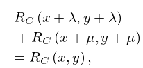
§19.26 Addition Theorems
… ►
19.26.11
…
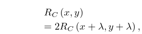
►The equations inverse to and the two other equations obtained by permuting (see (19.26.19)) are
…
►
19.26.25
.
…
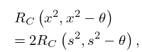
►
19.26.27
, or .
17: 3.11 Approximation Techniques
…
►
3.11.6
.
…
►
Laplace Transform Inversion
►Numerical inversion of the Laplace transform (§1.14(iii)) … ►If , then is the Lagrange interpolation polynomial for the set (§3.3(i)). … ►For many applications a spline function is a more adaptable approximating tool than the Lagrange interpolation polynomial involving a comparable number of parameters; see §3.3(i), where a single polynomial is used for interpolating on the complete interval . …18: Bibliography L
…
►
Démonstration d’un Théoréme d’Arithmétique.
Nouveau Mém. Acad. Roy. Sci. Berlin, pp. 123–133 (French).
…
