Lagrange formula for equally-spaced nodes

SearchAdvancedHelp

(0.004 seconds)

1—10 of 246 matching pages

1: 3.4 Differentiation

… ►

§3.4(i) Equally-Spaced Nodes

►The Lagrange $(n+1)$-point formula is … ►

Two-Point Formula

… ►For formulas for derivatives with equally-spaced real nodes and based on Sinc approximations (§3.3(vi)), see Stenger (1993, §3.5). …

2: 3.3 Interpolation

… ►

§3.3(i) Lagrange Interpolation

… ►The final expression in (3.3.1) is the Barycentric form of the Lagrange interpolation formula. … ►With an error term the Lagrange interpolation formula for $f$ is given by … ►

§3.3(ii) Lagrange Interpolation with Equally-Spaced Nodes

… ►

§3.3(iv) Newton’s Interpolation Formula

…

3: 2.2 Transcendental Equations

… ►where $F_0=f_0$ and $s{F}_s$ ($s\ge 1$) is the coefficient of $x^{-1}$ in the asymptotic expansion of ${(f(x))}^s$ (Lagrange’s formula for the reversion of series). …

4: 3.5 Quadrature

… ►The nodes $x_1,x_2,\mathrm{\dots },x_n$ are prescribed, and the weights $w_k$ and error term $E_n(f)$ are found by integrating the product of the Lagrange interpolation polynomial of degree $n-1$ and $w(x)$. … ► … ►

§3.5(v) Gauss Quadrature

… ►

Gauss–Laguerre Formula

… ►The nodes and weights of the 5-point complex Gauss quadrature formula (3.5.36) for $s=1$ are shown in Table 3.5.18. …

5: 27.13 Functions

… ►Lagrange (1770) proves that $g\left(2\right)=4$, and during the next 139 years the existence of $g\left(k\right)$ was shown for $k=3,4,5,6,7,8,10$. …A general formula states that … ►Explicit formulas for $r_k\left(n\right)$ have been obtained by similar methods for $k=6,8,10$, and $12$, but they are more complicated. Exact formulas for $r_k\left(n\right)$ have also been found for $k=3,5$, and $7$, and for all even $k\le 24$. …Also, Milne (1996, 2002) announce new infinite families of explicit formulas extending Jacobi’s identities. …

6: Bibliography G

… ►

Contiguous relations and summation and transformation formulae for basic hypergeometric series. J. Difference Equ. Appl. 19 (12), pp. 2029–2042.

ⓘ

External Links:

ISSN 1023-6198, Document, FullText, MathReview (Thomas Britz), ZentralBlatt

Referenced by:

§17.7(iii).

Encodings:

BibTeX

… ►

Formulas of the Dirichlet-Mehler Type. In Fractional Calculus and its Applications, B. Ross (Ed.), Lecture Notes in Math., Vol. 457, pp. 207–215.

ⓘ

External Links:

MathReview (Mourad E. H. Ismail), ZentralBlatt

Referenced by:

§18.10(i).

Encodings:

BibTeX

… ►

Construction of Gauss-Christoffel quadrature formulas. Math. Comp. 22, pp. 251–270.

ⓘ

External Links:

ISSN 0025-5718, Document, Link, MathReview (R. E. Barnhill)

Referenced by:

§18.39(iii).

Encodings:

BibTeX

… ►

On mean convergence of extended Lagrange interpolation. J. Comput. Appl. Math. 43 (1-2), pp. 19–35.

ⓘ

Notes:

Orthogonal polynomials and numerical methods

External Links:

ISSN 0377-0427, Document, Link, MathReview (Mircea Ivan), ZentralBlatt

Referenced by:

Erratum (V1.0.28) for Table 18.3.1.

Encodings:

BibTeX

… ►

Explicit formulas for Bernoulli numbers. Amer. Math. Monthly 79, pp. 44–51.

ⓘ

External Links:

FullText, MathReview (B. M. Stewart), ZentralBlatt

Referenced by:

§24.15(iii), §24.6.

Encodings:

BibTeX

…

7: 18.40 Methods of Computation

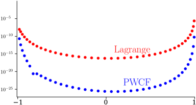
… ►In what follows this is accomplished in two ways: i) via the Lagrange interpolation of §3.3(i) ; and ii) by constructing a pointwise continued fraction, or PWCF, as follows: … ►Comparisons of the precisions of Lagrange and PWCF interpolations to obtain the derivatives, are shown in Figure 18.40.2. … ►

►►

Figure 18.40.2: Derivative Rule inversions for $w^{\mathrm{RCP}}(x)$ carried out via Lagrange and PWCF interpolations. …For the derivative rule Lagrange interpolation (red points) gives $\sim 15$ digits in the central region, while PWCF interpolation (blue points) gives $\sim 25$. Magnify

…

8: Bibliography D

… ►

A simple sum formula for Clebsch-Gordan coefficients. Lett. Math. Phys. 5 (3), pp. 207–211.

ⓘ

External Links:

ISSN 0377-9017, Document, MathReview, ZentralBlatt

Referenced by:

§14.17(iv).

Encodings:

BibTeX

… ►

Oscillatory integrals, Lagrange immersions and unfolding of singularities. Comm. Pure Appl. Math. 27, pp. 207–281.

ⓘ

External Links:

MathReview (Alan Weinstein), ZentralBlatt

Referenced by:

§36.12(iii).

Encodings:

BibTeX

… ►

Product formulas and Nicholson-type integrals for Jacobi functions. I. Summary of results. SIAM J. Math. Anal. 9 (1), pp. 76–86.

ⓘ

External Links:

Document, MathReview (R. C. Varma), ZentralBlatt

Referenced by:

§18.17(iii).

Encodings:

BibTeX

…

9: Bibliography B

… ►

Mathieu functions of general order: Connection formulae, base functions and asymptotic formulae. I–V. Philos. Trans. Roy. Soc. London Ser. A 301, pp. 75–162.

ⓘ

External Links:

ISSN 0080-4614, FullText, MathReview (J. Meixner), ZentralBlatt

Referenced by:

§28.8(iv).

Encodings:

BibTeX

… ►

Character analogues of the Poisson and Euler-MacLaurin summation formulas with applications. J. Number Theory 7 (4), pp. 413–445.

ⓘ

External Links:

Document, MathReview (T. M. Apostol), ZentralBlatt

Referenced by:

§24.16(ii).

Encodings:

BibTeX

►

Periodic Bernoulli numbers, summation formulas and applications. In Theory and Application of Special Functions (Proc. Advanced Sem., Math. Res. Center, Univ. Wisconsin, Madison, Wis., 1975), pp. 143–189.

ⓘ

External Links:

MathReview (L. Carlitz), ZentralBlatt

Referenced by:

§24.16(iii), §24.8(ii).

Encodings:

BibTeX

… ►

Barycentric Lagrange interpolation. SIAM Rev. 46 (3), pp. 501–517.

ⓘ

External Links:

ISSN 0036-1445, Document, Link, MathReview (Mao Dong Ye), ZentralBlatt

Referenced by:

§3.3(i).

Encodings:

BibTeX

… ►

A uniform asymptotic formula for orthogonal polynomials associated with $\exp (-x^4)$ . J. Approx. Theory 98, pp. 146–166.

ⓘ

External Links:

ISSN 0021-9045, Document, MathReview (V. L. Deshpande), ZentralBlatt

Referenced by:

§18.32.

Encodings:

BibTeX

…

10: 3.11 Approximation Techniques

… ►If $J=n+1$, then $p_n(x)$ is the Lagrange interpolation polynomial for the set $x_1,x_2,\mathrm{\dots },x_J$ (§3.3(i)). … ►Given $n+1$ distinct points $x_k$ in the real interval $[a,b]$, with ($a=$)($=b$), on each subinterval $[x_k,x_{k+1}]$, $k=0,1,\mathrm{\dots },n-1$, a low-degree polynomial is defined with coefficients determined by, for example, values $f_k$ and $f_k^{\prime }$ of a function $f$ and its derivative at the nodes $x_k$ and $x_{k+1}$. … ►For many applications a spline function is a more adaptable approximating tool than the Lagrange interpolation polynomial involving a comparable number of parameters; see §3.3(i), where a single polynomial is used for interpolating $f(x)$ on the complete interval $[a,b]$. …