L’Hôpital rule

SearchAdvancedHelp

(0.001 seconds)

11—20 of 134 matching pages

11: 18.41 Tables

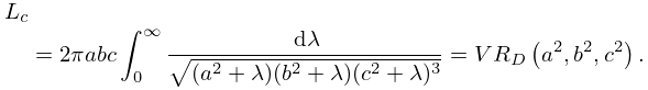
… ►Abramowitz and Stegun (1964, Tables 22.4, 22.6, 22.11, and 22.13) tabulates $T_n\left(x\right)$, $U_n\left(x\right)$, $L_n\left(x\right)$, and $H_n\left(x\right)$ for $n=0(1)12$. The ranges of $x$ are $0.2(.2)1$ for $T_n\left(x\right)$ and $U_n\left(x\right)$, and $0.5,1,3,5,10$ for $L_n\left(x\right)$ and $H_n\left(x\right)$. … ►For $P_n\left(x\right)$, $L_n\left(x\right)$, and $H_n\left(x\right)$ see §3.5(v). …

12: Bibliography

… ►

Numerical computation of Tricomi’s psi function by the trapezoidal rule. Computing 39 (3), pp. 271–279.

ⓘ

External Links:

ISSN 0010-485X, Document, MathReview, ZentralBlatt

Referenced by:

§13.29(iii).

Encodings:

BibTeX

►

Numerical evaluation of the Kummer function with complex argument by the trapezoidal rule. Rend. Sem. Mat. Univ. Politec. Torino 49 (3), pp. 315–327.

ⓘ

External Links:

ISSN 0373-1243, MathReview, ZentralBlatt

Referenced by:

§13.29(iii).

Encodings:

BibTeX

►

Numerical calculation of incomplete gamma functions by the trapezoidal rule. Numer. Math. 50 (4), pp. 419–428.

ⓘ

External Links:

ISSN 0029-599X, Document, MathReview (F. W. J. Olver), ZentralBlatt

Referenced by:

§8.25(ii).

Encodings:

BibTeX

… ►

Derivatives and integrals with respect to the order of the Struve functions ${𝐇}_{\nu }(x)$ and ${𝐋}_{\nu }(x)$ . J. Math. Anal. Appl. 137 (1), pp. 17–36.

ⓘ

External Links:

ISSN 0022-247X, Document, MathReview (A. McD. Mercer), ZentralBlatt

Referenced by:

§11.4(vi), §11.7(iv).

Encodings:

BibTeX

… ►

Note on the trivial zeros of Dirichlet $L$-functions. Proc. Amer. Math. Soc. 94 (1), pp. 29–30.

ⓘ

External Links:

ISSN 0002-9939, FullText, MathReview (Jerzy Kaczorowski), ZentralBlatt

Referenced by:

(25.15.7), (25.15.8), §25.15(ii), §25.15.

Encodings:

BibTeX

…

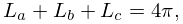
13: 19.33 Triaxial Ellipsoids

… ►The external field and the induced magnetization together produce a uniform field inside the ellipsoid with strength $H/(1+L_c\chi )$, where $L_c$ is the demagnetizing factor, given in cgs units by ►

19.33.7 $$L_c=2\pi abc{\int }_0^{\mathrm{\infty }}\frac{d\lambda }{\sqrt{(a^2+\lambda )(b^2+\lambda ){(c^2+\lambda )}^3}}=V{R}_D(a^2,b^2,c^2).$$

ⓘ

Symbols:

$R_D(x,y,z)$: elliptic integral symmetric in only two variables, $\pi$: the ratio of the circumference of a circle to its diameter, $dx$: differential of $x$ , $\int$: integral, $L_a$, $L_b$: factor and $V$: volume

Referenced by:

§19.15, §19.33(iii)

Permalink:

http://dlmf.nist.gov/19.33.E7

Encodings:

pMML, png, TeX

See also:

Annotations for §19.33(iii), §19.33 and Ch.19

… ►

19.33.8 $$L_a+L_b+L_c=4\pi ,$$

ⓘ

Symbols:

$\pi$: the ratio of the circumference of a circle to its diameter and $L_a$, $L_b$: factor

Permalink:

http://dlmf.nist.gov/19.33.E8

Encodings:

pMML, png, TeX

See also:

Annotations for §19.33(iii), §19.33 and Ch.19

►where $L_a$ and $L_b$ are obtained from $L_c$ by permutation of $a$, $b$, and $c$. …

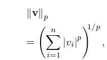
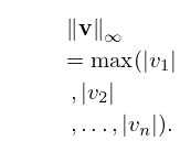
14: 1.2 Elementary Algebra

… ►This is the row times column rule. … ►

1.2.45 $${\Vert 𝐯\Vert }_p={\left(\sum _{i=1}^n{\left|v_i\right|}^p\right)}^{1/p},$$ $p\ge 1$.

ⓘ

Defines:

${\Vert 𝐯\Vert }_p$: L-p norm

Symbols:

$n$: nonnegative integer, $𝐯$: column vector and $\left|x\right|$: absolute value of $x$

Permalink:

http://dlmf.nist.gov/1.2.E45

Encodings:

pMML, png, TeX

See also:

Annotations for §1.2(v), §1.2(v), §1.2 and Ch.1

… ►

1.2.48 $${\Vert 𝐯\Vert }_{\mathrm{\infty }}=\max (\left|v_1\right|,\left|v_2\right|,\mathrm{\dots },\left|v_n\right|).$$

ⓘ

Defines:

${\Vert 𝐯\Vert }_{\mathrm{\infty }}$: l-infinity norm

Symbols:

$n$: nonnegative integer, $𝐯$: column vector and $\left|x\right|$: absolute value of $x$

Permalink:

http://dlmf.nist.gov/1.2.E48

Encodings:

pMML, png, TeX

See also:

Annotations for §1.2(v), §1.2(v), §1.2 and Ch.1

… ►

1.2.50 $$\left|⟨𝐮,𝐯⟩\right|\le {\Vert 𝐮\Vert }_p{\Vert 𝐯\Vert }_q,$$

ⓘ

Symbols:

${\Vert 𝐯\Vert }_p$: L-p norm, $⟨𝐮,𝐯⟩$: inner product over vectors, $𝐯$: column vector, $𝐮$: column vector and $\left|x\right|$: absolute value of $x$

Permalink:

http://dlmf.nist.gov/1.2.E50

Encodings:

pMML, png, TeX

See also:

Annotations for §1.2(v), §1.2(v), §1.2 and Ch.1

…

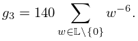
15: 23.9 Laurent and Other Power Series

… ►

23.9.1 $$c_n=(2n-1)\sum _{w\in 𝕃\setminus \{0\}}{w}^{-2n},$$ $n=2,3,4,\mathrm{\dots }$.

ⓘ

Symbols:

$\in$: element of, $\setminus$: set subtraction, $𝕃$: lattice, $n$: integer and $c_n$

Referenced by:

§20.6

Permalink:

http://dlmf.nist.gov/23.9.E1

Encodings:

pMML, png, TeX

See also:

Annotations for §23.9 and Ch.23

… ►

23.9.2 $$\mathrm{\wp }\left(z\right)=\frac{1}{z^2}+\sum _{n=2}^{\mathrm{\infty }}{c}_n{z}^{2n-2},$$ ,

ⓘ

Symbols:

$\mathrm{\wp }\left(z\right)$ (= $\mathrm{\wp }\left(z|𝕃\right)$ = $\mathrm{\wp }(z;g_2,g_3)$): Weierstrass $\mathrm{\wp }$-function, $𝕃$: lattice, $n$: integer, $z$: complex and $c_n$

A&S Ref:

18.5.1

Referenced by:

§23.9, §23.9

Permalink:

http://dlmf.nist.gov/23.9.E2

Encodings:

pMML, png, TeX

See also:

Annotations for §23.9 and Ch.23

►

23.9.3 $$\zeta \left(z\right)=\frac{1}{z}-\sum _{n=2}^{\mathrm{\infty }}\frac{c_n}{2n-1}{z}^{2n-1},$$ .

ⓘ

Symbols:

$\zeta \left(z\right)$ (= $\zeta \left(z|𝕃\right)$ = $\zeta (z;g_2,g_3)$): Weierstrass zeta function, $𝕃$: lattice, $n$: integer, $z$: complex and $c_n$

A&S Ref:

18.5.5

Referenced by:

§23.9

Permalink:

http://dlmf.nist.gov/23.9.E3

Encodings:

pMML, png, TeX

See also:

Annotations for §23.9 and Ch.23

… ►

23.9.6 $$\mathrm{\wp }\left({\omega }_j+t\right)=e_j+(3{e_j}^2-5c_2)t^2+(10c_2{e}_j+21c_3)t^4+(7c_2{e_j}^2+21c_3{e}_j+5c_2^2)t^6+O\left(t^8\right),$$

ⓘ

Symbols:

$O\left(x\right)$: order not exceeding, $\mathrm{\wp }\left(z\right)$ (= $\mathrm{\wp }\left(z|𝕃\right)$ = $\mathrm{\wp }(z;g_2,g_3)$): Weierstrass $\mathrm{\wp }$-function, $e_j$: Weierstrass lattice roots, $𝕃$: lattice, ${\omega }_1$, ${\omega }_3$, ${\omega }_2=-{\omega }_1-{\omega }_3$: lattice generators, $c_n$ and $t$: variable

Referenced by:

§23.9

Permalink:

http://dlmf.nist.gov/23.9.E6

Encodings:

pMML, png, TeX

See also:

Annotations for §23.9 and Ch.23

… ►

23.9.7 $$\sigma \left(z\right)=\sum _{m,n=0}^{\mathrm{\infty }}{a}_{m,n}{(10c_2)}^m{(56c_3)}^n\frac{z^{4m+6n+1}}{(4m+6n+1)!},$$

ⓘ

Symbols:

$\sigma \left(z\right)$ (= $\sigma \left(z|𝕃\right)$ = $\sigma (z;g_2,g_3)$): Weierstrass sigma function, $!$: factorial (as in $n!$), $𝕃$: lattice, $n$: integer, $m$: integer, $z$: complex, $c_n$ and $a_{m,n}$: coefficients

A&S Ref:

18.5.6

Referenced by:

§23.9

Permalink:

http://dlmf.nist.gov/23.9.E7

Encodings:

pMML, png, TeX

See also:

Annotations for §23.9 and Ch.23

…

16: 11.15 Approximations

… ►

Luke (1975, pp. 416–421) gives Chebyshev-series expansions for ${𝐇}_n\left(x\right)$, ${𝐋}_n\left(x\right)$, $0\le \left|x\right|\le 8$, and ${𝐇}_n\left(x\right)-Y_n\left(x\right)$, $x\ge 8$, for $n=0,1$; ${\int }_0^x{t}^{-m}{𝐇}_0\left(t\right)dt$, ${\int }_0^x{t}^{-m}{𝐋}_0\left(t\right)dt$, $0\le \left|x\right|\le 8$, $m=0,1$ and ${\int }_0^x({𝐇}_0\left(t\right)-Y_0\left(t\right))dt$, ${\int }_x^{\mathrm{\infty }}{t}^{-1}({𝐇}_0\left(t\right)-Y_0\left(t\right))dt$, $x\ge 8$; the coefficients are to 20D.

►

MacLeod (1993) gives Chebyshev-series expansions for ${𝐋}_0\left(x\right)$, ${𝐋}_1\left(x\right)$, $0\le x\le 16$, and $I_0\left(x\right)-{𝐋}_0\left(x\right)$, $I_1\left(x\right)-{𝐋}_1\left(x\right)$, $x\ge 16$; the coefficients are to 20D.

…

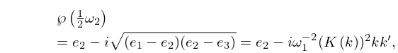
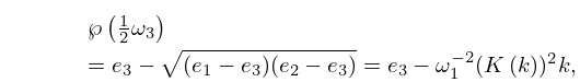
17: 23.7 Quarter Periods

… ►

23.7.1 $$\mathrm{\wp }\left(\frac{1}{2}{\omega }_1\right)=e_1+\sqrt{(e_1-e_3)(e_1-e_2)}=e_1+{\omega }_1^{-2}{(K\left(k\right))}^2{k}^{\prime },$$

ⓘ

Symbols:

$\mathrm{\wp }\left(z\right)$ (= $\mathrm{\wp }\left(z|𝕃\right)$ = $\mathrm{\wp }(z;g_2,g_3)$): Weierstrass $\mathrm{\wp }$-function, $e_j$: Weierstrass lattice roots, $K\left(k\right)$: Legendre’s complete elliptic integral of the first kind, $𝕃$: lattice, ${\omega }_1$, ${\omega }_3$, ${\omega }_2=-{\omega }_1-{\omega }_3$: lattice generators, $k$: modulus and $k^{\prime }$: complementary modulus

A&S Ref:

18.3.18

Permalink:

http://dlmf.nist.gov/23.7.E1

Encodings:

pMML, png, TeX

See also:

Annotations for §23.7 and Ch.23

►

23.7.2 $$\mathrm{\wp }\left(\frac{1}{2}{\omega }_2\right)=e_2-\mathrm{i}\sqrt{(e_1-e_2)(e_2-e_3)}=e_2-\mathrm{i}{\omega }_1^{-2}{(K\left(k\right))}^{2}k{k}^{\prime },$$

ⓘ

Symbols:

$\mathrm{\wp }\left(z\right)$ (= $\mathrm{\wp }\left(z|𝕃\right)$ = $\mathrm{\wp }(z;g_2,g_3)$): Weierstrass $\mathrm{\wp }$-function, $e_j$: Weierstrass lattice roots, $K\left(k\right)$: Legendre’s complete elliptic integral of the first kind, $\mathrm{i}$: imaginary unit, $𝕃$: lattice, ${\omega }_1$, ${\omega }_3$, ${\omega }_2=-{\omega }_1-{\omega }_3$: lattice generators, $k$: modulus and $k^{\prime }$: complementary modulus

A&S Ref:

18.3.18

Permalink:

http://dlmf.nist.gov/23.7.E2

Encodings:

pMML, png, TeX

See also:

Annotations for §23.7 and Ch.23

►

23.7.3 $$\mathrm{\wp }\left(\frac{1}{2}{\omega }_3\right)=e_3-\sqrt{(e_1-e_3)(e_2-e_3)}=e_3-{\omega }_1^{-2}{(K\left(k\right))}^{2}k,$$

ⓘ

Symbols:

$\mathrm{\wp }\left(z\right)$ (= $\mathrm{\wp }\left(z|𝕃\right)$ = $\mathrm{\wp }(z;g_2,g_3)$): Weierstrass $\mathrm{\wp }$-function, $e_j$: Weierstrass lattice roots, $K\left(k\right)$: Legendre’s complete elliptic integral of the first kind, $𝕃$: lattice, ${\omega }_1$, ${\omega }_3$, ${\omega }_2=-{\omega }_1-{\omega }_3$: lattice generators and $k$: modulus

A&S Ref:

18.3.18

Permalink:

http://dlmf.nist.gov/23.7.E3

Encodings:

pMML, png, TeX

See also:

Annotations for §23.7 and Ch.23

…

18: 18.8 Differential Equations

… ►

Table 18.8.1: Classical OP’s: differential equations $A(x)f^{\prime \prime }(x)+B(x)f^{\prime }(x)+C(x)f(x)+{\lambda }_{n}f(x)=0$.

► ►►►►►►

#	$f(x)$	$A(x)$	$B(x)$	$C(x)$	${\lambda }_n$
…
8	$L_n^{(\alpha )}\left(x\right)$	$x$	$\alpha +1-x$	$0$	$n$
9	${\mathrm{e}}^{-\frac{1}{2}{x}^2}{x}^{\alpha +\frac{1}{2}}{L}_n^{(\alpha )}\left(x^2\right)$	$1$	$0$	$-x^2+(\frac{1}{4}-{\alpha }^2)x^{-2}$	$4n+2\alpha +2$
10	${\mathrm{e}}^{-\frac{1}{2}x}{x}^{\frac{1}{2}\alpha }{L}_n^{(\alpha )}\left(x\right)$	$x$	$1$	$-\frac{1}{4}x-\frac{1}{4}{\alpha }^2{x}^{-1}$	$n+\frac{1}{2}(\alpha +1)$
11	${\mathrm{e}}^{-n^{-1}x}{x}^{\mathrm{\ell }+1}{L}_{n-\mathrm{\ell }-1}^{(2\mathrm{\ell }+1)}\left(2n^{-1}x\right)$	$1$	$0$	$\frac{2}{x}-\frac{\mathrm{\ell }(\mathrm{\ell }+1)}{x^2}$	$-\frac{1}{n^2}$
…

►

…

19: 23.3 Differential Equations

… ►

23.3.1 $$g_2=60\sum _{w\in 𝕃\setminus \{0\}}{w}^{-4},$$

ⓘ

Symbols:

$g_j$: Weierstrass lattice invariants $g_2$, $g_3$ , $\in$: element of, $\setminus$: set subtraction and $𝕃$: lattice

A&S Ref:

18.1.1

Referenced by:

§23.3(i)

Permalink:

http://dlmf.nist.gov/23.3.E1

Encodings:

pMML, png, TeX

See also:

Annotations for §23.3(i), §23.3 and Ch.23

►

23.3.2 $$g_3=140\sum _{w\in 𝕃\setminus \{0\}}{w}^{-6}.$$

ⓘ

Symbols:

$g_j$: Weierstrass lattice invariants $g_2$, $g_3$ , $\in$: element of, $\setminus$: set subtraction and $𝕃$: lattice

A&S Ref:

18.1.1

Referenced by:

§23.3(i)

Permalink:

http://dlmf.nist.gov/23.3.E2

Encodings:

pMML, png, TeX

See also:

Annotations for §23.3(i), §23.3 and Ch.23

… ►Given $g_2$ and $g_3$ there is a unique lattice $𝕃$ such that (23.3.1) and (23.3.2) are satisfied. … ►Conversely, $g_2$, $g_3$, and the set $\{e_1,e_2,e_3\}$ are determined uniquely by the lattice $𝕃$ independently of the choice of generators. However, given any pair of generators $2{\omega }_1$, $2{\omega }_3$ of $𝕃$, and with ${\omega }_2$ defined by (23.2.1), we can identify the $e_j$ individually, via …

20: 3.11 Approximation Techniques

… ►to the maximum error of the minimax polynomial $p_n(x)$ is bounded by $1+L_n$, where $L_n$ is the $n$th Lebesgue constant for Fourier series; see §1.8(i). Since $L_0=1$, $L_n$ is a monotonically increasing function of $n$, and (for example) $L_{1000}=4.07\mathrm{\dots }$, this means that in practice the gain in replacing a truncated Chebyshev-series expansion by the corresponding minimax polynomial approximation is hardly worthwhile. … ►The Padé approximants can be computed by Wynn’s cross rule. Any five approximants arranged in the Padé table as …