L%E2%80%99H%C3%B4pital%20rule

SearchAdvancedHelp

Did you mean L%E2%80%99H%C3%hopital%20rule ?

(0.003 seconds)

1—10 of 325 matching pages

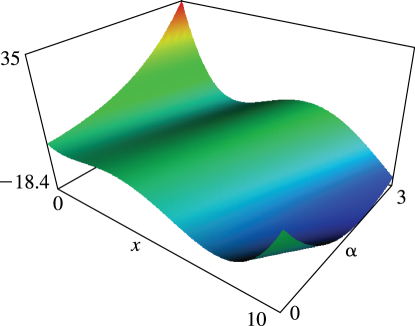
1: 18.4 Graphics

… ►

►►

Figure 18.4.5: Laguerre polynomials $L_n\left(x\right)$, $n=1,2,3,4,5$. Magnify

►

►►

Figure 18.4.6: Laguerre polynomials $L_3^{(\alpha )}\left(x\right)$, $\alpha =0,1,2,3,4$. Magnify

►

►►

Figure 18.4.7: Monic Hermite polynomials $h_n(x)=2^{-n}{H}_n\left(x\right)$, $n=1,2,3,4,5$. Magnify

… ►

►

►

Figure 18.4.8: Laguerre polynomials $L_3^{(\alpha )}\left(x\right)$, $0\le \alpha \le 3$, $0\le x\le 10$. Magnify 3D Help

►

►

►

Figure 18.4.9: Laguerre polynomials $L_4^{(\alpha )}\left(x\right)$, $0\le \alpha \le 3$, $0\le x\le 10$. Magnify 3D Help

2: 18.36 Miscellaneous Polynomials

… ►

§18.36(v) Non-Classical Laguerre Polynomials $L_n^{(-k)}\left(x\right)$, $k=1,2\mathrm{\dots }$

… ►For the Laguerre polynomials $L_n^{(\alpha )}\left(x\right)$ this requires, omitting all strictly positive factors, … ►implying that, for $n\ge k$, the orthogonality of the $L_n^{(-k)}\left(x\right)$ with respect to the Laguerre weight function $x^{-k}{\mathrm{e}}^{-x}$, $x\in [0,\mathrm{\infty })$. …These results are proven in Everitt et al. (2004), via construction of a self-adjoint Sturm–Liouville operator which generates the $L_n^{(-k)}(x)$ polynomials, self-adjointness implying both orthogonality and completeness. … ►The resulting EOP’s, ${\widehat{L}}_n^{(k)}\left(x\right)$, $n=1,2,\mathrm{\dots }$ satisfy …

3: 23.14 Integrals

… ►

23.14.1 $$\int \mathrm{\wp }\left(z\right)dz=-\zeta \left(z\right),$$

ⓘ

Symbols:

$\mathrm{\wp }\left(z\right)$ (= $\mathrm{\wp }\left(z|𝕃\right)$ = $\mathrm{\wp }(z;g_2,g_3)$): Weierstrass $\mathrm{\wp }$-function, $\zeta \left(z\right)$ (= $\zeta \left(z|𝕃\right)$ = $\zeta (z;g_2,g_3)$): Weierstrass zeta function, $dx$: differential of $x$ , $\int$: integral, $𝕃$: lattice and $z$: complex

A&S Ref:

18.6.1

Permalink:

http://dlmf.nist.gov/23.14.E1

Encodings:

pMML, png, TeX

See also:

Annotations for §23.14 and Ch.23

►

23.14.2 $$\int {\mathrm{\wp }}^2\left(z\right)dz=\frac{1}{6}{\mathrm{\wp }}^{\prime }\left(z\right)+\frac{1}{12}{g}_{2}z,$$

ⓘ

Symbols:

$\mathrm{\wp }\left(z\right)$ (= $\mathrm{\wp }\left(z|𝕃\right)$ = $\mathrm{\wp }(z;g_2,g_3)$): Weierstrass $\mathrm{\wp }$-function, $g_j$: Weierstrass lattice invariants $g_2$, $g_3$ , $dx$: differential of $x$ , $\int$: integral, $𝕃$: lattice and $z$: complex

A&S Ref:

18.7.1

Permalink:

http://dlmf.nist.gov/23.14.E2

Encodings:

pMML, png, TeX

See also:

Annotations for §23.14 and Ch.23

►

23.14.3 $$\int {\mathrm{\wp }}^3\left(z\right)dz=\frac{1}{120}{\mathrm{\wp }}^{\prime \prime \prime }\left(z\right)-\frac{3}{20}{g}_2\zeta \left(z\right)+\frac{1}{10}{g}_{3}z.$$

ⓘ

Symbols:

$\mathrm{\wp }\left(z\right)$ (= $\mathrm{\wp }\left(z|𝕃\right)$ = $\mathrm{\wp }(z;g_2,g_3)$): Weierstrass $\mathrm{\wp }$-function, $g_j$: Weierstrass lattice invariants $g_2$, $g_3$ , $\zeta \left(z\right)$ (= $\zeta \left(z|𝕃\right)$ = $\zeta (z;g_2,g_3)$): Weierstrass zeta function, $dx$: differential of $x$ , $\int$: integral, $𝕃$: lattice and $z$: complex

A&S Ref:

18.7.2

Permalink:

http://dlmf.nist.gov/23.14.E3

Encodings:

pMML, png, TeX

See also:

Annotations for §23.14 and Ch.23

…

4: 18.41 Tables

… ►Abramowitz and Stegun (1964, Tables 22.4, 22.6, 22.11, and 22.13) tabulates $T_n\left(x\right)$, $U_n\left(x\right)$, $L_n\left(x\right)$, and $H_n\left(x\right)$ for $n=0(1)12$. The ranges of $x$ are $0.2(.2)1$ for $T_n\left(x\right)$ and $U_n\left(x\right)$, and $0.5,1,3,5,10$ for $L_n\left(x\right)$ and $H_n\left(x\right)$. The precision is 10D, except for $H_n\left(x\right)$ which is 6-11S. … ►For $P_n\left(x\right)$, $L_n\left(x\right)$, and $H_n\left(x\right)$ see §3.5(v). …

5: 11.14 Tables

… ►

Abramowitz and Stegun (1964, Chapter 12) tabulates ${𝐇}_n\left(x\right)$, ${𝐇}_n\left(x\right)-Y_n\left(x\right)$, and $I_n\left(x\right)-{𝐋}_n\left(x\right)$ for $n=0,1$ and $x=0(.1)5$, $x^{-1}=0(.01)0.2$ to 6D or 7D.

►

Agrest et al. (1982) tabulates ${𝐇}_n\left(x\right)$ and ${\mathrm{e}}^{-x}{𝐋}_n\left(x\right)$ for $n=0,1$ and $x=0(.001)5(.005)15(.01)100$ to 11D.

… ►

Zhang and Jin (1996) tabulates ${𝐇}_n\left(x\right)$ and ${𝐋}_n\left(x\right)$ for $n=-4(1)3$ and $x=0(1)20$ to 8D or 7S.

… ►

Abramowitz and Stegun (1964, Chapter 12) tabulates ${\int }_0^x(I_0\left(t\right)-{𝐋}_0\left(t\right))dt$ and $(2/\pi ){\int }_x^{\mathrm{\infty }}{t}^{-1}{𝐇}_0\left(t\right)dt$ for $x=0(.1)5$ to 5D or 7D; ${\int }_0^x({𝐇}_0\left(t\right)-Y_0\left(t\right))dt-(2/\pi )\ln x$, ${\int }_0^x(I_0\left(t\right)-{𝐋}_0\left(t\right))dt-(2/\pi )\ln x$, and ${\int }_x^{\mathrm{\infty }}{t}^{-1}({𝐇}_0\left(t\right)-Y_0\left(t\right))dt$ for $x^{-1}=0(.01)0.2$ to 6D.

►

Agrest et al. (1982) tabulates ${\int }_0^x{𝐇}_0\left(t\right)dt$ and ${\mathrm{e}}^{-x}{\int }_0^x{𝐋}_0\left(t\right)dt$ for $x=0(.001)5(.005)15(.01)100$ to 11D.

…

6: 11.15 Approximations

… ►

Luke (1975, pp. 416–421) gives Chebyshev-series expansions for ${𝐇}_n\left(x\right)$, ${𝐋}_n\left(x\right)$, $0\le \left|x\right|\le 8$, and ${𝐇}_n\left(x\right)-Y_n\left(x\right)$, $x\ge 8$, for $n=0,1$; ${\int }_0^x{t}^{-m}{𝐇}_0\left(t\right)dt$, ${\int }_0^x{t}^{-m}{𝐋}_0\left(t\right)dt$, $0\le \left|x\right|\le 8$, $m=0,1$ and ${\int }_0^x({𝐇}_0\left(t\right)-Y_0\left(t\right))dt$, ${\int }_x^{\mathrm{\infty }}{t}^{-1}({𝐇}_0\left(t\right)-Y_0\left(t\right))dt$, $x\ge 8$; the coefficients are to 20D.

►

MacLeod (1993) gives Chebyshev-series expansions for ${𝐋}_0\left(x\right)$, ${𝐋}_1\left(x\right)$, $0\le x\le 16$, and $I_0\left(x\right)-{𝐋}_0\left(x\right)$, $I_1\left(x\right)-{𝐋}_1\left(x\right)$, $x\ge 16$; the coefficients are to 20D.

… ►

Newman (1984) gives polynomial approximations for ${𝐇}_n\left(x\right)$ for $n=0,1$, $0\le x\le 3$, and rational-fraction approximations for ${𝐇}_n\left(x\right)-Y_n\left(x\right)$ for $n=0,1$, $x\ge 3$. The maximum errors do not exceed 1.2×10⁻⁸ for the former and 2.5×10⁻⁸ for the latter.

7: 19.33 Triaxial Ellipsoids

… ►Let a homogeneous magnetic ellipsoid with semiaxes $a,b,c$, volume $V=4\pi abc/3$, and susceptibility $\chi$ be placed in a previously uniform magnetic field $H$ parallel to the principal axis with semiaxis $c$. The external field and the induced magnetization together produce a uniform field inside the ellipsoid with strength $H/(1+L_c\chi )$, where $L_c$ is the demagnetizing factor, given in cgs units by ►

19.33.7 $$L_c=2\pi abc{\int }_0^{\mathrm{\infty }}\frac{d\lambda }{\sqrt{(a^2+\lambda )(b^2+\lambda ){(c^2+\lambda )}^3}}=V{R}_D(a^2,b^2,c^2).$$

ⓘ

Symbols:

$R_D(x,y,z)$: elliptic integral symmetric in only two variables, $\pi$: the ratio of the circumference of a circle to its diameter, $dx$: differential of $x$ , $\int$: integral, $L_a$, $L_b$: factor and $V$: volume

Referenced by:

§19.15, §19.33(iii)

Permalink:

http://dlmf.nist.gov/19.33.E7

Encodings:

pMML, png, TeX

See also:

Annotations for §19.33(iii), §19.33 and Ch.19

… ►

19.33.8 $$L_a+L_b+L_c=4\pi ,$$

ⓘ

Symbols:

$\pi$: the ratio of the circumference of a circle to its diameter and $L_a$, $L_b$: factor

Permalink:

http://dlmf.nist.gov/19.33.E8

Encodings:

pMML, png, TeX

See also:

Annotations for §19.33(iii), §19.33 and Ch.19

►where $L_a$ and $L_b$ are obtained from $L_c$ by permutation of $a$, $b$, and $c$. …

8: 23.9 Laurent and Other Power Series

… ►

23.9.1 $$c_n=(2n-1)\sum _{w\in 𝕃\setminus \{0\}}{w}^{-2n},$$ $n=2,3,4,\mathrm{\dots }$.

ⓘ

Symbols:

$\in$: element of, $\setminus$: set subtraction, $𝕃$: lattice, $n$: integer and $c_n$

Referenced by:

§20.6

Permalink:

http://dlmf.nist.gov/23.9.E1

Encodings:

pMML, png, TeX

See also:

Annotations for §23.9 and Ch.23

… ►

23.9.2 $$\mathrm{\wp }\left(z\right)=\frac{1}{z^2}+\sum _{n=2}^{\mathrm{\infty }}{c}_n{z}^{2n-2},$$ ,

ⓘ

Symbols:

$\mathrm{\wp }\left(z\right)$ (= $\mathrm{\wp }\left(z|𝕃\right)$ = $\mathrm{\wp }(z;g_2,g_3)$): Weierstrass $\mathrm{\wp }$-function, $𝕃$: lattice, $n$: integer, $z$: complex and $c_n$

A&S Ref:

18.5.1

Referenced by:

§23.9, §23.9

Permalink:

http://dlmf.nist.gov/23.9.E2

Encodings:

pMML, png, TeX

See also:

Annotations for §23.9 and Ch.23

►

23.9.3 $$\zeta \left(z\right)=\frac{1}{z}-\sum _{n=2}^{\mathrm{\infty }}\frac{c_n}{2n-1}{z}^{2n-1},$$ .

ⓘ

Symbols:

$\zeta \left(z\right)$ (= $\zeta \left(z|𝕃\right)$ = $\zeta (z;g_2,g_3)$): Weierstrass zeta function, $𝕃$: lattice, $n$: integer, $z$: complex and $c_n$

A&S Ref:

18.5.5

Referenced by:

§23.9

Permalink:

http://dlmf.nist.gov/23.9.E3

Encodings:

pMML, png, TeX

See also:

Annotations for §23.9 and Ch.23

… ►

23.9.6 $$\mathrm{\wp }\left({\omega }_j+t\right)=e_j+(3{e_j}^2-5c_2)t^2+(10c_2{e}_j+21c_3)t^4+(7c_2{e_j}^2+21c_3{e}_j+5c_2^2)t^6+O\left(t^8\right),$$

ⓘ

Symbols:

$O\left(x\right)$: order not exceeding, $\mathrm{\wp }\left(z\right)$ (= $\mathrm{\wp }\left(z|𝕃\right)$ = $\mathrm{\wp }(z;g_2,g_3)$): Weierstrass $\mathrm{\wp }$-function, $e_j$: Weierstrass lattice roots, $𝕃$: lattice, ${\omega }_1$, ${\omega }_3$, ${\omega }_2=-{\omega }_1-{\omega }_3$: lattice generators, $c_n$ and $t$: variable

Referenced by:

§23.9

Permalink:

http://dlmf.nist.gov/23.9.E6

Encodings:

pMML, png, TeX

See also:

Annotations for §23.9 and Ch.23

… ►

23.9.7 $$\sigma \left(z\right)=\sum _{m,n=0}^{\mathrm{\infty }}{a}_{m,n}{(10c_2)}^m{(56c_3)}^n\frac{z^{4m+6n+1}}{(4m+6n+1)!},$$

ⓘ

Symbols:

$\sigma \left(z\right)$ (= $\sigma \left(z|𝕃\right)$ = $\sigma (z;g_2,g_3)$): Weierstrass sigma function, $!$: factorial (as in $n!$), $𝕃$: lattice, $n$: integer, $m$: integer, $z$: complex, $c_n$ and $a_{m,n}$: coefficients

A&S Ref:

18.5.6

Referenced by:

§23.9

Permalink:

http://dlmf.nist.gov/23.9.E7

Encodings:

pMML, png, TeX

See also:

Annotations for §23.9 and Ch.23

…

9: 18.8 Differential Equations

… ►

Table 18.8.1: Classical OP’s: differential equations $A(x)f^{\prime \prime }(x)+B(x)f^{\prime }(x)+C(x)f(x)+{\lambda }_{n}f(x)=0$.

► ►►►►►►►

#	$f(x)$	$A(x)$	$B(x)$	$C(x)$	${\lambda }_n$
…
8	$L_n^{(\alpha )}\left(x\right)$	$x$	$\alpha +1-x$	$0$	$n$
9	${\mathrm{e}}^{-\frac{1}{2}{x}^2}{x}^{\alpha +\frac{1}{2}}{L}_n^{(\alpha )}\left(x^2\right)$	$1$	$0$	$-x^2+(\frac{1}{4}-{\alpha }^2)x^{-2}$	$4n+2\alpha +2$
10	${\mathrm{e}}^{-\frac{1}{2}x}{x}^{\frac{1}{2}\alpha }{L}_n^{(\alpha )}\left(x\right)$	$x$	$1$	$-\frac{1}{4}x-\frac{1}{4}{\alpha }^2{x}^{-1}$	$n+\frac{1}{2}(\alpha +1)$
11	${\mathrm{e}}^{-n^{-1}x}{x}^{\mathrm{\ell }+1}{L}_{n-\mathrm{\ell }-1}^{(2\mathrm{\ell }+1)}\left(2n^{-1}x\right)$	$1$	$0$	$\frac{2}{x}-\frac{\mathrm{\ell }(\mathrm{\ell }+1)}{x^2}$	$-\frac{1}{n^2}$
12	$H_n\left(x\right)$	$1$	$-2x$	$0$	$2n$
…

►

…

10: 18.5 Explicit Representations

… ►Similarly in the cases of the ultraspherical polynomials $C_n^{(\lambda )}\left(x\right)$ and the Laguerre polynomials $L_n^{(\alpha )}\left(x\right)$ we assume that $\lambda >-\frac{1}{2},\lambda \ne 0$, and $\alpha >-1$, unless stated otherwise. … ►

$L_0\left(x\right)=1,$

… ►

$L_6\left(x\right)=\frac{1}{720}{x}^6-\frac{1}{20}{x}^5+\frac{5}{8}{x}^4-\frac{10}{3}{x}^3+\frac{15}{2}{x}^2-6x+1.$

►

$L_0^{(\alpha )}\left(x\right)=1,$

►

$L_1^{(\alpha )}\left(x\right)=-x+\alpha +1,$

…