L orthornormal basis

SearchAdvancedHelp

Did you mean L orthonormal basis ?

(0.002 seconds)

1—10 of 113 matching pages

1: 23.21 Physical Applications

… ►In §22.19(ii) it is noted that Jacobian elliptic functions provide a natural basis of solutions for problems in Newtonian classical dynamics with quartic potentials in canonical form $(1-x^2)(1-k^2{x}^2)$. … ►

23.21.1 $$\frac{x^2}{\rho -e_1}+\frac{y^2}{\rho -e_2}+\frac{z^2}{\rho -e_3}=1,$$

ⓘ

Symbols:

$e_j$: Weierstrass lattice roots, $𝕃$: lattice, $x$: real part of $z$ , $y$: imaginary part of $z$ , $z$: complex and $\rho$: roots

Permalink:

http://dlmf.nist.gov/23.21.E1

Encodings:

pMML, png, TeX

See also:

Annotations for §23.21(iii), §23.21 and Ch.23

… ►

23.21.3 $$f(\rho )=2{\left((\rho -e_1)(\rho -e_2)(\rho -e_3)\right)}^{1/2}.$$

ⓘ

Symbols:

$e_j$: Weierstrass lattice roots, $𝕃$: lattice, $\rho$: roots and $f(\rho )$: function

Permalink:

http://dlmf.nist.gov/23.21.E3

Encodings:

pMML, png, TeX

See also:

Annotations for §23.21(iii), §23.21 and Ch.23

… ►

23.21.5 $$\left(\mathrm{\wp }\left(v\right)-\mathrm{\wp }\left(w\right)\right)\left(\mathrm{\wp }\left(w\right)-\mathrm{\wp }\left(u\right)\right)\left(\mathrm{\wp }\left(u\right)-\mathrm{\wp }\left(v\right)\right){\nabla }^2=\left(\mathrm{\wp }\left(w\right)-\mathrm{\wp }\left(v\right)\right)\frac{{\partial }^2}{{\partial u}^2}+\left(\mathrm{\wp }\left(u\right)-\mathrm{\wp }\left(w\right)\right)\frac{{\partial }^2}{{\partial v}^2}+\left(\mathrm{\wp }\left(v\right)-\mathrm{\wp }\left(u\right)\right)\frac{{\partial }^2}{{\partial w}^2}.$$

ⓘ

Symbols:

$\mathrm{\wp }\left(z\right)$ (= $\mathrm{\wp }\left(z|𝕃\right)$ = $\mathrm{\wp }(z;g_2,g_3)$): Weierstrass $\mathrm{\wp }$-function, $\frac{\partial f}{\partial x}$: partial derivative of $f$ with respect to $x$ , $\partial x$: partial differential of $x$ , $𝕃$: lattice, $u$: change of variable, $v$: change of variable and $w$: change of variable

Permalink:

http://dlmf.nist.gov/23.21.E5

Encodings:

pMML, png, TeX

See also:

Annotations for §23.21(iii), §23.21 and Ch.23

…

2: 18.39 Applications in the Physical Sciences

… ►where ${\mathrm{L}}^2$ is the (squared) angular momentum operator (14.30.12). … ►with an infinite set of orthonormal $L^2$ eigenfunctions … ►is tridiagonalized in the complete $L^2$ non-orthogonal (with measure $dr$, $r\in [0,\mathrm{\infty })$) basis of Laguerre functions: … ►For either sign of $Z$, and $s$ chosen such that $n+l+1+(2Z/s)>0$, $n=0,1,2,\mathrm{\dots }$, truncation of the basis to $N$ terms, with $x_i^N\in [-1,1]$, the discrete eigenvectors are the orthonormal $L^2$ functions …This equivalent quadrature relationship, see Heller et al. (1973), Yamani and Reinhardt (1975), allows extraction of scattering information from the finite dimensional $L^2$ functions of (18.39.53), provided that such information involves potentials, or projections onto $L^2$ functions, exactly expressed, or well approximated, in the finite basis of (18.39.44). …

3: 25.15 Dirichlet $L$-functions

§25.15 Dirichlet $L$-functions

►

§25.15(i) Definitions and Basic Properties

►The notation $L(s,\chi )$ was introduced by Dirichlet (1837) for the meromorphic continuation of the function defined by the series … … ►

§25.15(ii) Zeros

…

4: 1.18 Linear Second Order Differential Operators and Eigenfunction Expansions

… ►

§1.18(ii) $L^2$ spaces on intervals in $ℝ$

… ►Assume that ${\left\{{\varphi }_n\right\}}_{n=0}^{\mathrm{\infty }}$ is an orthonormal basis of $L^2\left(X\right)$. …where the limit has to be understood in the sense of $L^2$ convergence in the mean: … ►The eigenfunctions form a complete orthogonal basis in $L^2\left(X\right)$, and we can take the basis as orthonormal: … ►Eigenfunctions corresponding to the continuous spectrum are non-$L^2$ functions. …

5: 31.15 Stieltjes Polynomials

… ►

31.15.12

ⓘ

Defines:

$\rho (z)$: weight function (locally)

Symbols:

$z$: complex variable, $\gamma$: real or complex parameter, $j$: nonnegative integer, $a$: complex parameter and $N+1$: number of singularities

Permalink:

http://dlmf.nist.gov/31.15.E12

Encodings:

pMML, png, TeX

See also:

Annotations for §31.15(iii), §31.15 and Ch.31

►The normalized system of products (31.15.8) forms an orthonormal basis in the Hilbert space $L_{\rho }^2(Q)$. For further details and for the expansions of analytic functions in this basis see Volkmer (1999).

6: 18.4 Graphics

… ►

►►

Figure 18.4.5: Laguerre polynomials $L_n\left(x\right)$, $n=1,2,3,4,5$. Magnify

►

►►

Figure 18.4.6: Laguerre polynomials $L_3^{(\alpha )}\left(x\right)$, $\alpha =0,1,2,3,4$. Magnify

… ►

►

►

Figure 18.4.8: Laguerre polynomials $L_3^{(\alpha )}\left(x\right)$, $0\le \alpha \le 3$, $0\le x\le 10$. Magnify 3D Help

►

►

►

Figure 18.4.9: Laguerre polynomials $L_4^{(\alpha )}\left(x\right)$, $0\le \alpha \le 3$, $0\le x\le 10$. Magnify 3D Help

7: 30.15 Signal Analysis

… ►The sequence ${\varphi }_n$, $n=0,1,2,\mathrm{\dots }$ forms an orthonormal basis in the space of $\sigma$-bandlimited functions, and, after normalization, an orthonormal basis in $L^2(-\tau ,\tau )$. … ►taken over all $f\in L^2(-\mathrm{\infty },\mathrm{\infty })$ subject to …

8: 23.10 Addition Theorems and Other Identities

… ►

23.10.10 $$\sigma \left(2z\right)=-{\mathrm{\wp }}^{\prime }\left(z\right){\sigma }^4\left(z\right).$$

ⓘ

Symbols:

$\mathrm{\wp }\left(z\right)$ (= $\mathrm{\wp }\left(z|𝕃\right)$ = $\mathrm{\wp }(z;g_2,g_3)$): Weierstrass $\mathrm{\wp }$-function, $\sigma \left(z\right)$ (= $\sigma \left(z|𝕃\right)$ = $\sigma (z;g_2,g_3)$): Weierstrass sigma function, $𝕃$: lattice and $z$: complex

A&S Ref:

18.4.8

Referenced by:

§23.10(ii)

Permalink:

http://dlmf.nist.gov/23.10.E10

Encodings:

pMML, png, TeX

See also:

Annotations for §23.10(ii), §23.10 and Ch.23

… ►

23.10.17 $$\mathrm{\wp }\left(cz|c𝕃\right)=c^{-2}\mathrm{\wp }\left(z|𝕃\right),$$

ⓘ

Symbols:

$\mathrm{\wp }\left(z\right)$ (= $\mathrm{\wp }\left(z|𝕃\right)$ = $\mathrm{\wp }(z;g_2,g_3)$): Weierstrass $\mathrm{\wp }$-function, $𝕃$: lattice, $z$: complex and $c$: constant

A&S Ref:

18.2.2

Permalink:

http://dlmf.nist.gov/23.10.E17

Encodings:

pMML, png, TeX

See also:

Annotations for §23.10(iv), §23.10 and Ch.23

►

23.10.18 $$\zeta \left(cz|c𝕃\right)=c^{-1}\zeta \left(z|𝕃\right),$$

ⓘ

Symbols:

$\zeta \left(z\right)$ (= $\zeta \left(z|𝕃\right)$ = $\zeta (z;g_2,g_3)$): Weierstrass zeta function, $𝕃$: lattice, $z$: complex and $c$: constant

A&S Ref:

18.2.3

Permalink:

http://dlmf.nist.gov/23.10.E18

Encodings:

pMML, png, TeX

See also:

Annotations for §23.10(iv), §23.10 and Ch.23

►

23.10.19 $$\sigma \left(cz|c𝕃\right)=c\sigma \left(z|𝕃\right).$$

ⓘ

Symbols:

$\sigma \left(z\right)$ (= $\sigma \left(z|𝕃\right)$ = $\sigma (z;g_2,g_3)$): Weierstrass sigma function, $𝕃$: lattice, $z$: complex and $c$: constant

A&S Ref:

18.2.4

Permalink:

http://dlmf.nist.gov/23.10.E19

Encodings:

pMML, png, TeX

See also:

Annotations for §23.10(iv), §23.10 and Ch.23

►Also, when $𝕃$ is replaced by $c𝕃$ the lattice invariants $g_2$ and $g_3$ are divided by $c^4$ and $c^6$, respectively. …

9: 18.36 Miscellaneous Polynomials

… ►

§18.36(v) Non-Classical Laguerre Polynomials $L_n^{(-k)}\left(x\right)$, $k=1,2\mathrm{\dots }$

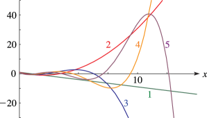
… ►For the Laguerre polynomials $L_n^{(\alpha )}\left(x\right)$ this requires, omitting all strictly positive factors, … ►implying that, for $n\ge k$, the orthogonality of the $L_n^{(-k)}\left(x\right)$ with respect to the Laguerre weight function $x^{-k}{\mathrm{e}}^{-x}$, $x\in [0,\mathrm{\infty })$. …These results are proven in Everitt et al. (2004), via construction of a self-adjoint Sturm–Liouville operator which generates the $L_n^{(-k)}(x)$ polynomials, self-adjointness implying both orthogonality and completeness. 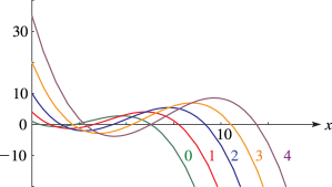… ►The resulting EOP’s, ${\widehat{L}}_n^{(k)}\left(x\right)$, $n=1,2,\mathrm{\dots }$ satisfy …

10: 23.14 Integrals

… ►

23.14.1 $$\int \mathrm{\wp }\left(z\right)dz=-\zeta \left(z\right),$$

ⓘ

Symbols:

$\mathrm{\wp }\left(z\right)$ (= $\mathrm{\wp }\left(z|𝕃\right)$ = $\mathrm{\wp }(z;g_2,g_3)$): Weierstrass $\mathrm{\wp }$-function, $\zeta \left(z\right)$ (= $\zeta \left(z|𝕃\right)$ = $\zeta (z;g_2,g_3)$): Weierstrass zeta function, $dx$: differential of $x$ , $\int$: integral, $𝕃$: lattice and $z$: complex

A&S Ref:

18.6.1

Permalink:

http://dlmf.nist.gov/23.14.E1

Encodings:

pMML, png, TeX

See also:

Annotations for §23.14 and Ch.23

►

23.14.2 $$\int {\mathrm{\wp }}^2\left(z\right)dz=\frac{1}{6}{\mathrm{\wp }}^{\prime }\left(z\right)+\frac{1}{12}{g}_{2}z,$$

ⓘ

Symbols:

$\mathrm{\wp }\left(z\right)$ (= $\mathrm{\wp }\left(z|𝕃\right)$ = $\mathrm{\wp }(z;g_2,g_3)$): Weierstrass $\mathrm{\wp }$-function, $g_j$: Weierstrass lattice invariants $g_2$, $g_3$ , $dx$: differential of $x$ , $\int$: integral, $𝕃$: lattice and $z$: complex

A&S Ref:

18.7.1

Permalink:

http://dlmf.nist.gov/23.14.E2

Encodings:

pMML, png, TeX

See also:

Annotations for §23.14 and Ch.23

►

23.14.3 $$\int {\mathrm{\wp }}^3\left(z\right)dz=\frac{1}{120}{\mathrm{\wp }}^{\prime \prime \prime }\left(z\right)-\frac{3}{20}{g}_2\zeta \left(z\right)+\frac{1}{10}{g}_{3}z.$$

ⓘ

Symbols:

$\mathrm{\wp }\left(z\right)$ (= $\mathrm{\wp }\left(z|𝕃\right)$ = $\mathrm{\wp }(z;g_2,g_3)$): Weierstrass $\mathrm{\wp }$-function, $g_j$: Weierstrass lattice invariants $g_2$, $g_3$ , $\zeta \left(z\right)$ (= $\zeta \left(z|𝕃\right)$ = $\zeta (z;g_2,g_3)$): Weierstrass zeta function, $dx$: differential of $x$ , $\int$: integral, $𝕃$: lattice and $z$: complex

A&S Ref:

18.7.2

Permalink:

http://dlmf.nist.gov/23.14.E3

Encodings:

pMML, png, TeX

See also:

Annotations for §23.14 and Ch.23

…