Kummer transformation

SearchAdvancedHelp

(0.001 seconds)

11—20 of 24 matching pages

11: Bibliography M

… ►

On a Kummer-type transformation for the generalized hypergeometric function ${}_2{}^{}F_2^{}$ . J. Comput. Appl. Math. 157 (2), pp. 507–509.

ⓘ

External Links:

ISSN 0377-0427, Document, MathReview Entry, ZentralBlatt

Referenced by:

§16.6.

Encodings:

BibTeX

…

12: Bibliography C

… ►

An extension of a Kummer’s quadratic transformation formula with an application. Proc. Jangjeon Math. Soc. 16 (2), pp. 229–235.

ⓘ

External Links:

ISSN 1598-7264, MathReview (Petr Blaschke), ZentralBlatt

Referenced by:

§16.6, §16.6.

Encodings:

BibTeX

…

13: 18.17 Integrals

… ►

§18.17(v) Fourier Transforms

… ►

Jacobi

… ►

Ultraspherical

… ►

§18.17(vi) Laplace Transforms

… ►

§18.17(vii) Mellin Transforms

…

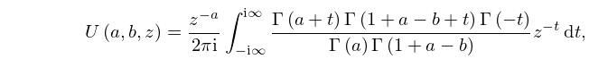
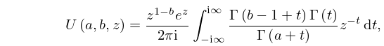
14: 13.4 Integral Representations

… ►

13.4.16 $$𝐌(a,b,-z)=\frac{1}{2\pi \mathrm{i}\mathrm{\Gamma }\left(a\right)}{\int }_{-\mathrm{i}\mathrm{\infty }}^{\mathrm{i}\mathrm{\infty }}\frac{\mathrm{\Gamma }\left(a+t\right)\mathrm{\Gamma }\left(-t\right)}{\mathrm{\Gamma }\left(b+t\right)}{z}^{t}dt,$$ ,

ⓘ

Symbols:

$\mathrm{\Gamma }\left(z\right)$: gamma function, $𝐌(a,b,z)$: Olver’s confluent hypergeometric function, $\pi$: the ratio of the circumference of a circle to its diameter, $dx$: differential of $x$ , $\mathrm{i}$: imaginary unit, $\int$: integral, $\mathrm{ph}$: phase and $z$: complex variable

Keywords:

Mellin transform

A&S Ref:

13.2.9 (in different form)

Permalink:

http://dlmf.nist.gov/13.4.E16

Encodings:

pMML, png, TeX

See also:

Annotations for §13.4(iii), §13.4 and Ch.13

… ►

13.4.17 $$U(a,b,z)=\frac{z^{-a}}{2\pi \mathrm{i}}{\int }_{-\mathrm{i}\mathrm{\infty }}^{\mathrm{i}\mathrm{\infty }}\frac{\mathrm{\Gamma }\left(a+t\right)\mathrm{\Gamma }\left(1+a-b+t\right)\mathrm{\Gamma }\left(-t\right)}{\mathrm{\Gamma }\left(a\right)\mathrm{\Gamma }\left(1+a-b\right)}{z}^{-t}dt,$$ ,

ⓘ

Symbols:

$\mathrm{\Gamma }\left(z\right)$: gamma function, $U(a,b,z)$: Kummer confluent hypergeometric function, $\pi$: the ratio of the circumference of a circle to its diameter, $dx$: differential of $x$ , $\mathrm{i}$: imaginary unit, $\int$: integral, $\mathrm{ph}$: phase and $z$: complex variable

Keywords:

Mellin transform

A&S Ref:

13.2.10

Referenced by:

§13.6(vi)

Permalink:

http://dlmf.nist.gov/13.4.E17

Encodings:

pMML, png, TeX

See also:

Annotations for §13.4(iii), §13.4 and Ch.13

… ►

13.4.18 $$U(a,b,z)=\frac{z^{1-b}{\mathrm{e}}^z}{2\pi \mathrm{i}}{\int }_{-\mathrm{i}\mathrm{\infty }}^{\mathrm{i}\mathrm{\infty }}\frac{\mathrm{\Gamma }\left(b-1+t\right)\mathrm{\Gamma }\left(t\right)}{\mathrm{\Gamma }\left(a+t\right)}{z}^{-t}dt,$$ ,

ⓘ

Symbols:

$\mathrm{\Gamma }\left(z\right)$: gamma function, $U(a,b,z)$: Kummer confluent hypergeometric function, $\pi$: the ratio of the circumference of a circle to its diameter, $dx$: differential of $x$ , $\mathrm{e}$: base of natural logarithm, $\mathrm{i}$: imaginary unit, $\int$: integral, $\mathrm{ph}$: phase and $z$: complex variable

Keywords:

Mellin transform

Permalink:

http://dlmf.nist.gov/13.4.E18

Encodings:

pMML, png, TeX

See also:

Annotations for §13.4(iii), §13.4 and Ch.13

…

15: Bibliography T

… ►

Asymptotic expansions of Kummer hypergeometric functions for large values of the parameters. Integral Transforms Spec. Funct. 33 (1), pp. 16–31.

ⓘ

External Links:

ISSN 1065-2469, Document, Link, MathReview Entry, ZentralBlatt

Referenced by:

§13.8(iv).

Encodings:

BibTeX

…

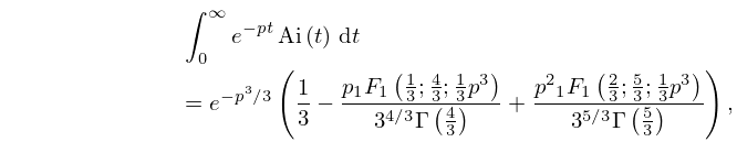
16: 9.10 Integrals

… ►

9.10.14 $${\int }_0^{\mathrm{\infty }}{\mathrm{e}}^{-pt}\mathrm{Ai}\left(t\right)dt={\mathrm{e}}^{-p^3/3}\left(\frac{1}{3}-\frac{p{}_1{}^{}F_1^{}(\frac{1}{3};\frac{4}{3};\frac{1}{3}{p}^3)}{3^{4/3}\mathrm{\Gamma }\left(\frac{4}{3}\right)}+\frac{p^2{}_1{}^{}F_1^{}(\frac{2}{3};\frac{5}{3};\frac{1}{3}{p}^3)}{3^{5/3}\mathrm{\Gamma }\left(\frac{5}{3}\right)}\right),$$ $p\in ℂ$.

ⓘ

Symbols:

$\mathrm{Ai}\left(z\right)$: Airy function, $\mathrm{\Gamma }\left(z\right)$: gamma function, ${}_1{}^{}F_1^{}(a;b;z)$: $=M(a,b,z)$ notation for the Kummer confluent hypergeometric function, $ℂ$: complex plane, $dx$: differential of $x$ , $\in$: element of, $\mathrm{e}$: base of natural logarithm, $\int$: integral and $p$: parameter

Keywords:

Laplace transform

Source:

Gibbs (1973, Problem 72–21)

Permalink:

http://dlmf.nist.gov/9.10.E14

Encodings:

pMML, png, TeX

See also:

Annotations for §9.10(v), §9.10 and Ch.9

…

17: 15.10 Hypergeometric Differential Equation

… ►The three pairs of fundamental solutions given by (15.10.2), (15.10.4), and (15.10.6) can be transformed into 18 other solutions by means of (15.8.1), leading to a total of 24 solutions known as Kummer’s solutions. …

18: Bibliography D

… ►

Integral Transforms and their Applications. 2nd edition, Applied Mathematical Sciences, Vol. 25, Springer-Verlag, New York.

ⓘ

External Links:

ISBN 0-387-96080-5, MathReview, ZentralBlatt

Referenced by:

§1.14(vii).

Encodings:

BibTeX

… ►

Computational properties of three-term recurrence relations for Kummer functions. J. Comput. Appl. Math. 233 (6), pp. 1505–1510.

ⓘ

External Links:

ISSN 0377-0427, Document, FullText, MathReview (Richard B. Paris), ZentralBlatt

Referenced by:

§13.29(iv), §13.29(iv).

Encodings:

BibTeX

►

The Radon Transform and Some of Its Applications. A Wiley-Interscience Publication, John Wiley & Sons Inc., New York.

ⓘ

Notes:

Reprinted by Dover in 2007.

External Links:

ISBN 0-471-89804-X, MathReview (W. R. Madych), ZentralBlatt

Referenced by:

§18.38(ii).

Encodings:

BibTeX

►

Integral transforms and their applications. Third edition, CRC Press, Boca Raton, FL.

ⓘ

External Links:

ISBN 978-1-4822-2357-6, MathReview Entry, ZentralBlatt

Referenced by:

§1.16(viii).

Encodings:

BibTeX

… ►

Handbuch der Laplace-Transformation. Bd. II. Anwendungen der Laplace-Transformation. 1. Abteilung. Birkhäuser Verlag, Basel und Stuttgart (German).

ⓘ

External Links:

MathReview (I. I. Hirschman), ZentralBlatt

Referenced by:

§2.5(i).

Encodings:

BibTeX

…

19: Bibliography Z

… ►

Distribution of zeros of Gauss and Kummer hypergeometric functions. A semiclassical approach. Ann. Numer. Math. 2 (1-4), pp. 457–472.

ⓘ

External Links:

ISSN 1021-2655, MathReview (B. D. Agrawal), ZentralBlatt

Referenced by:

§13.9(i), §15.13.

Encodings:

BibTeX

… ►

Distribution Theory and Transform Analysis, An Introduction and Generalized Functions with Applications. Dover, New York.

ⓘ

Notes:

Reprint of 1965 McGraw-Hill Publication

External Links:

ISBN 0-486-65479-6, MathReview Entry

Referenced by:

§1.16(ix).

Encodings:

BibTeX

… ►

Generalized Watson Transforms and Applications to Group Representations. Ph.D. Thesis, University of Vermont, Burlington,VT.

ⓘ

Referenced by:

§35.7(ii).

Encodings:

BibTeX

►

A fast Fourier-Bessel transform algorithm. Zh. Vychisl. Mat. i Mat. Fiz. 35 (7), pp. 1128–1133 (Russian).

ⓘ

Notes:

English translation in Comput. Math. Math. Phys. 35(7), pp. 901–905

External Links:

ISSN 0044-4669, MathReview (Vítĕzslav Veselý), ZentralBlatt

Referenced by:

§10.74(vii).

Encodings:

BibTeX

…

20: Errata

… ►

A note about the multivalued nature of the Kummer confluent hypergeometric function of the second kind $U$ on the right-hand side of (7.18.10) was inserted.

… ►

There have been extensive changes in the notation used for the integral transforms defined in §1.14. These changes are applied throughout the DLMF. The following table summarizes the changes.

Transform	New	Abbreviated	Old
	Notation	Notation	Notation
Fourier	$ℱ\left(f\right)\left(x\right)$	$ℱf\left(x\right)$
Fourier Cosine	${ℱ}_c\left(f\right)\left(x\right)$	${ℱ}_{c}f\left(x\right)$
Fourier Sine	${ℱ}_s\left(f\right)\left(x\right)$	${ℱ}_{s}f\left(x\right)$
Laplace	$ℒ\left(f\right)\left(s\right)$	$ℒf\left(s\right)$	$ℒ(f(t);s)$
Mellin	$ℳ\left(f\right)\left(s\right)$	$ℳf\left(s\right)$	$ℳ(f;s)$
Hilbert	$\mathscr{H}\left(f\right)\left(s\right)$	$\mathscr{H}f\left(s\right)$	$\mathscr{H}(f;s)$
Stieltjes	$𝒮\left(f\right)\left(s\right)$	$𝒮f\left(s\right)$	$𝒮(f;s)$

Previously, for the Fourier, Fourier cosine and Fourier sine transforms, either temporary local notations were used or the Fourier integrals were written out explicitly.

… ►

There were clarifications made in the conditions on the parameter $a$ in $U(a,b,z)$ of those equations.

… ►

13.2.7 $$U(-m,b,z)={(-1)}^m{\left(b\right)}_{m}M(-m,b,z)={(-1)}^m\sum _{s=0}^m\left(\genfrac{}{}{0.0pt}{}{m}{s}\right){\left(b+s\right)}_{m-s}{(-z)}^s$$

The equality $U(-m,b,z)={(-1)}^m{\left(b\right)}_{m}M(-m,b,z)$ has been added to the original equation to express an explicit connection between the two standard solutions of Kummer’s equation. Note also that the notation $a=-n$ has been changed to $a=-m$.

Reported 2015-02-10 by Adri Olde Daalhuis.

►

13.2.8 $$U(a,a+n+1,z)=\frac{{(-1)}^n{\left(1-a-n\right)}_n}{z^{a+n}}M(-n,1-a-n,z)=z^{-a}\sum _{s=0}^n\left(\genfrac{}{}{0.0pt}{}{n}{s}\right){\left(a\right)}_s{z}^{-s}$$

The equality $U(a,a+n+1,z)=\frac{{(-1)}^n{\left(1-a-n\right)}_n}{z^{a+n}}M(-n,1-a-n,z)$ has been added to the original equation to express an explicit connection between the two standard solutions of Kummer’s equation.

Reported 2015-02-10 by Adri Olde Daalhuis.

…