Julia%20sets

SearchAdvancedHelp

(0.003 seconds)

1—10 of 605 matching pages

1: 3.8 Nonlinear Equations

… ►Consider $x=20$ and $j=19$. We have $p^{\prime }(20)=19!$ and $a_{19}=1+2+\mathrm{\cdots }+20=210$. … ►It is called a Julia set. In general the Julia set of an analytic function $f(z)$ is a fractal, that is, a set that is self-similar. See Julia (1918) and Devaney (1986). …

2: Bibliography J

… ►

Note sur la série ${\sum }_{n=1}^{\mathrm{\infty }}{x}^n/n^s$ . Bull. Soc. Math. France 17, pp. 142–152 (French).

ⓘ

External Links:

ISSN 0037-9484, MathReview Entry, ZentralBlatt

Referenced by:

§25.12(ii).

Encodings:

BibTeX

… ►

Memoire sur l’itération des fonctions rationnelles. J. Math. Pures Appl. 8 (1), pp. 47–245 (French).

ⓘ

External Links:

FullText, ZentralBlatt

Referenced by:

§3.8(viii).

Encodings:

BibTeX

3: 20 Theta Functions

Chapter 20 Theta Functions

…

4: William P. Reinhardt

… ►Reinhardt firmly believes that the Mandelbrot set is a special function, and notes with interest that the natural boundaries of analyticity of many “more normal” special functions are also fractals. … ►

20 Theta Functions

… ►In November 2015, Reinhardt was named Senior Associate Editor of the DLMF and Associate Editor for Chapters 20, 22, and 23.

5: 36.5 Stokes Sets

§36.5 Stokes Sets

►

§36.5(i) Definitions

… ►

§36.5(ii) Cuspoids

… ►

Elliptic Umbilic Stokes Set (Codimension three)

… ►

§36.5(iv) Visualizations

…

6: 10.75 Tables

… ►

The main tables in Abramowitz and Stegun (1964, Chapter 9) give $J_0\left(x\right)$ to 15D, $J_1\left(x\right)$, $J_2\left(x\right)$, $Y_0\left(x\right)$, $Y_1\left(x\right)$ to 10D, $Y_2\left(x\right)$ to 8D, $x=0(.1)17.5$; $Y_n\left(x\right)-(2/\pi )J_n\left(x\right)\ln x$, $n=0,1$, $x=0(.1)2$, 8D; $J_n\left(x\right)$, $Y_n\left(x\right)$, $n=3(1)9$, $x=0(.2)20$, 5D or 5S; $J_n\left(x\right)$, $Y_n\left(x\right)$, $n=0(1)20(10)50,100$, $x=1,2,5,10,50,100$, 10S; modulus and phase functions $\sqrt{x}{M}_n\left(x\right)$, ${\theta }_n\left(x\right)-x$, $n=0,1,2$, $1/x=0(.01)0.1$, 8D.

►

Achenbach (1986) tabulates $J_0\left(x\right)$, $J_1\left(x\right)$, $Y_0\left(x\right)$, $Y_1\left(x\right)$, $x=0(.1)8$, 20D or 18–20S.

… ►

Makinouchi (1966) tabulates all values of $j_{\nu ,m}$ and $y_{\nu ,m}$ in the interval $(0,100)$, with at least 29S. These are for $\nu =0(1)5$, 10, 20; $\nu =\frac{3}{2}$, $\frac{5}{2}$; $\nu =m/n$ with $m=1(1)n-1$ and $n=3(1)8$, except for $\nu =\frac{1}{2}$.

… ►

Bickley et al. (1952) tabulates $x^{-n}{I}_n\left(x\right)$ or ${\mathrm{e}}^{-x}{I}_n\left(x\right)$, $x^n{K}_n\left(x\right)$ or ${\mathrm{e}}^x{K}_n\left(x\right)$, $n=2(1)20$, $x=0$(.01 or .1) 10(.1) 20, 8S; $I_n\left(x\right)$, $K_n\left(x\right)$, $n=0(1)20$, $x=0$ or $0.1(.1)20$, 10S.

… ►

The main tables in Abramowitz and Stegun (1964, Chapter 9) give ${\mathrm{e}}^{-x}{I}_n\left(x\right)$, ${\mathrm{e}}^x{K}_n\left(x\right)$, $n=0,1,2$, $x=0(.1)10(.2)20$, 8D–10D or 10S; $\sqrt{x}{\mathrm{e}}^{-x}{I}_n\left(x\right)$, $(\sqrt{x}/\pi )$ ${\mathrm{e}}^x{K}_n\left(x\right)$, $n=0,1,2$, $1/x=0(.002)0.05$; $K_0\left(x\right)+I_0\left(x\right)\ln x$, $x(K_1\left(x\right)-I_1\left(x\right)\ln x)$, $x=0(.1)2$, 8D; ${\mathrm{e}}^{-x}{I}_n\left(x\right)$, ${\mathrm{e}}^x{K}_n\left(x\right)$, $n=3(1)9$, $x=0(.2)10(.5)20$, 5S; $I_n\left(x\right)$, $K_n\left(x\right)$, $n=0(1)20(10)50,100$, $x=1,2,5,10,50,100$, 9–10S.

…

7: 9.18 Tables

… ►

Miller (1946) tabulates $\mathrm{Ai}\left(x\right)$, ${\mathrm{Ai}}^{\prime }\left(x\right)$ for $x=-20(.01)2;$ ${\log }_{10}\mathrm{Ai}\left(x\right)$, ${\mathrm{Ai}}^{\prime }\left(x\right)/\mathrm{Ai}\left(x\right)$ for $x=0(.1)25(1)75$; $\mathrm{Bi}\left(x\right)$, ${\mathrm{Bi}}^{\prime }\left(x\right)$ for $x=-10(.1)2.5$; ${\log }_{10}\mathrm{Bi}\left(x\right)$, ${\mathrm{Bi}}^{\prime }\left(x\right)/\mathrm{Bi}\left(x\right)$ for $x=0(.1)10$; $M\left(x\right)$, $N\left(x\right)$, $\theta \left(x\right)$, $\varphi \left(x\right)$ (respectively $F(x)$, $G(x)$, $\chi (x)$, $\psi (x)$) for $x=-80(1)-30(.1)0$. Precision is generally 8D; slightly less for some of the auxiliary functions. Extracts from these tables are included in Abramowitz and Stegun (1964, Chapter 10), together with some auxiliary functions for large arguments.

►

Fox (1960, Table 3) tabulates $2{\pi }^{1/2}{x}^{1/4}\exp (\frac{2}{3}{x}^{3/2})\mathrm{Ai}\left(x\right)$, $2{\pi }^{1/2}{x}^{-1/4}\exp (\frac{2}{3}{x}^{3/2}){\mathrm{Ai}}^{\prime }\left(x\right)$, ${\pi }^{1/2}{x}^{1/4}\exp (-\frac{2}{3}{x}^{3/2})\mathrm{Bi}\left(x\right)$, and ${\pi }^{1/2}{x}^{-1/4}\exp (-\frac{2}{3}{x}^{3/2}){\mathrm{Bi}}^{\prime }\left(x\right)$ for $\frac{3}{2}{x}^{-3/2}=0(.001)0.05$, together with similar auxiliary functions for negative values of $x$. Precision is 10D.

►

Zhang and Jin (1996, p. 337) tabulates $\mathrm{Ai}\left(x\right)$, ${\mathrm{Ai}}^{\prime }\left(x\right)$, $\mathrm{Bi}\left(x\right)$, ${\mathrm{Bi}}^{\prime }\left(x\right)$ for $x=0(1)20$ to 8S and for $x=-20(1)0$ to 9D.

… ►

Miller (1946) tabulates $a_k$, ${\mathrm{Ai}}^{\prime }\left(a_k\right)$, $a_k^{\prime }$, $\mathrm{Ai}\left(a_k^{\prime }\right)$, $k=1(1)50$; $b_k$, ${\mathrm{Bi}}^{\prime }\left(b_k\right)$, $b_k^{\prime }$, $\mathrm{Bi}\left(b_k^{\prime }\right)$, $k=1(1)20$. Precision is 8D. Entries for $k=1(1)20$ are reproduced in Abramowitz and Stegun (1964, Chapter 10).

►

Sherry (1959) tabulates $a_k$, ${\mathrm{Ai}}^{\prime }\left(a_k\right)$, $a_k^{\prime }$, $\mathrm{Ai}\left(a_k^{\prime }\right)$, $k=1(1)50$; 20S.

…

8: 36.4 Bifurcation Sets

§36.4 Bifurcation Sets

… ►

Bifurcation (Catastrophe) Set for Cuspoids

… ►

Bifurcation (Catastrophe) Set for Umbilics

… ► $K=1$, fold bifurcation set: … ►

§36.4(ii) Visualizations

…

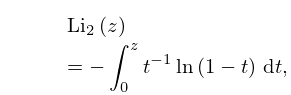
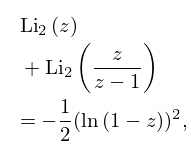
9: 25.12 Polylogarithms

… ►

25.12.2 $${\mathrm{Li}}_2\left(z\right)=-{\int }_0^z{t}^{-1}\ln \left(1-t\right)dt,$$ $z\in ℂ\setminus (1,\mathrm{\infty })$.

ⓘ

Symbols:

$ℂ$: complex plane, $dx$: differential of $x$ , ${\mathrm{Li}}_2\left(z\right)$: dilogarithm, $\in$: element of, $\int$: integral, $\ln z$: principal branch of logarithm function, $(a,b)$: open interval, $\setminus$: set subtraction, $x$: real variable and $z$: complex variable

Keywords:

definite integral, integral representation

Source:

Maximon (2003, (2.1), p. 2807)

A&S Ref:

27.7.1 (is a modified form with $z=1-x$)

Referenced by:

§25.12(i)

Permalink:

http://dlmf.nist.gov/25.12.E2

Encodings:

pMML, png, TeX

See also:

Annotations for §25.12(i), §25.12 and Ch.25

… ►

25.12.3 $${\mathrm{Li}}_2\left(z\right)+{\mathrm{Li}}_2\left(\frac{z}{z-1}\right)=-\frac{1}{2}{(\ln \left(1-z\right))}^2,$$ $z\in ℂ\setminus [1,\mathrm{\infty })$.

ⓘ

Symbols:

$[a,b)$: half-closed interval, $ℂ$: complex plane, ${\mathrm{Li}}_2\left(z\right)$: dilogarithm, $\in$: element of, $\ln z$: principal branch of logarithm function, $\setminus$: set subtraction, $x$: real variable and $z$: complex variable

Keywords:

connection formula

Source:

Maximon (2003, (3.4), p. 2808)

A&S Ref:

27.7.5 (is a modified form with $z=1-x$)

Permalink:

http://dlmf.nist.gov/25.12.E3

Encodings:

pMML, png, TeX

See also:

Annotations for §25.12(i), §25.12 and Ch.25

… ►

►►

Figure 25.12.1: Dilogarithm function ${\mathrm{Li}}_2\left(x\right)$, Magnify

►

►

►

Figure 25.12.2: Absolute value of the dilogarithm function $\left|{\mathrm{Li}}_2\left(x+\mathrm{i}y\right)\right|$, $-20\le x\le 20$, $-20\le y\le 20$. … Magnify 3D Help

… ►Sometimes the factor $1/\mathrm{\Gamma }\left(s+1\right)$ is omitted. …

10: 26.2 Basic Definitions

… ►A permutation is a one-to-one and onto function from a non-empty set to itself. If the set consists of the integers 1 through $n$, a permutation $\sigma$ can be thought of as a rearrangement of these integers where the integer in position $j$ is $\sigma (j)$. … ►Given a finite set $S$ with permutation $\sigma$, a cycle is an ordered equivalence class of elements of $S$ where $j$ is equivalent to $k$ if there exists an $\mathrm{\ell }=\mathrm{\ell }(j,k)$ such that $j={\sigma }^{\mathrm{\ell }}(k)$, where ${\sigma }^1=\sigma$ and ${\sigma }^{\mathrm{\ell }}$ is the composition of $\sigma$ with ${\sigma }^{\mathrm{\ell }-1}$. … ►

Partition

►A partition of a set $S$ is an unordered collection of pairwise disjoint nonempty sets whose union is $S$. …