Jacobi imaginary transformation

SearchAdvancedHelp

(0.003 seconds)

11—20 of 24 matching pages

11: 23.6 Relations to Other Functions

… ►

23.6.11 $$\sigma \left({\omega }_2\right)=-2{\omega }_1\frac{\exp \left(\frac{1}{2}{\eta }_1({\omega }_1{\tau }^2+{\omega }_3-{\omega }_2)\right){\theta }_3(0,q)}{\pi q^{1/4}{\theta }_1^{\prime }(0,q)},$$

ⓘ

Symbols:

${\theta }_j(z,q)$: theta function, $\sigma \left(z\right)$ (= $\sigma \left(z|𝕃\right)$ = $\sigma (z;g_2,g_3)$): Weierstrass sigma function, $\pi$: the ratio of the circumference of a circle to its diameter, $\exp z$: exponential function, $\mathrm{i}$: imaginary unit, $𝕃$: lattice, $q$: nome, ${\omega }_1$, ${\omega }_3$, ${\omega }_2=-{\omega }_1-{\omega }_3$: lattice generators, $\tau$: complex variable and ${\eta }_j$: complex number

Referenced by:

Erratum (V1.1.1) for Equation (23.6.11)

Permalink:

http://dlmf.nist.gov/23.6.E11

Encodings:

pMML, png, TeX

Correction (effective with 1.1.1):

The factor $2{\omega }_1\mathrm{i}\exp \left(\frac{1}{2}{\eta }_1{\omega }_1{\tau }^2\right)$ has been corrected to be $-2{\omega }_1\exp \left(\frac{1}{2}{\eta }_1({\omega }_1{\tau }^2+{\omega }_3-{\omega }_2)\right)$.

See also:

Annotations for §23.6(i), §23.6 and Ch.23

►

23.6.12 $$\sigma \left({\omega }_3\right)=2\mathrm{i}{\omega }_1\frac{\exp \left(\frac{1}{2}{\eta }_1{\omega }_1{\tau }^2\right){\theta }_4(0,q)}{\pi q^{1/4}{\theta }_1^{\prime }(0,q)}.$$

ⓘ

Symbols:

${\theta }_j(z,q)$: theta function, $\sigma \left(z\right)$ (= $\sigma \left(z|𝕃\right)$ = $\sigma (z;g_2,g_3)$): Weierstrass sigma function, $\pi$: the ratio of the circumference of a circle to its diameter, $\exp z$: exponential function, $\mathrm{i}$: imaginary unit, $𝕃$: lattice, $q$: nome, ${\omega }_1$, ${\omega }_3$, ${\omega }_2=-{\omega }_1-{\omega }_3$: lattice generators, $\tau$: complex variable and ${\eta }_j$: complex number

Referenced by:

§23.6(i), Erratum (V1.1.1) for Equation (23.6.12)

Permalink:

http://dlmf.nist.gov/23.6.E12

Encodings:

pMML, png, TeX

Correction (effective with 1.1.1):

The factor $-2{\omega }_1\exp \left(\frac{1}{2}{\eta }_1{\omega }_1\right)$ has been corrected to be $2\mathrm{i}{\omega }_1\exp \left(\frac{1}{2}{\eta }_1{\omega }_1{\tau }^2\right)$.

See also:

Annotations for §23.6(i), §23.6 and Ch.23

… ►Also, ${𝕃}_1$, ${𝕃}_2$, ${𝕃}_3$ are the lattices with generators $(4K,2\mathrm{i}{K}^{\prime })$, $(2K-2\mathrm{i}{K}^{\prime },2K+2\mathrm{i}{K}^{\prime })$, $(2K,4\mathrm{i}{K}^{\prime })$, respectively. … ►Similar results for the other nine Jacobi functions can be constructed with the aid of the transformations given by Table 22.4.3. ►For representations of the Jacobi functions $\mathrm{sn}$, $\mathrm{cn}$, and $\mathrm{dn}$ as quotients of $\sigma$-functions see Lawden (1989, §§6.2, 6.3). …

12: 22.17 Moduli Outside the Interval [0,1]

… ►

§22.17(i) Real or Purely Imaginary Moduli

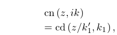
►Jacobian elliptic functions with real moduli in the intervals $(-\mathrm{\infty },0)$ and $(1,\mathrm{\infty })$, or with purely imaginary moduli are related to functions with moduli in the interval $[0,1]$ by the following formulas. … ►

22.17.7 $$\mathrm{cn}(z,\mathrm{i}k)=\mathrm{cd}(z/k_1^{\prime },k_1),$$

ⓘ

Symbols:

$\mathrm{cd}(z,k)$: Jacobian elliptic function, $\mathrm{cn}(z,k)$: Jacobian elliptic function, $\mathrm{i}$: imaginary unit, $z$: complex, $k$: modulus, $k_1$: change of variable and $k_1^{\prime }$: change of variable

A&S Ref:

16.10.3 (modified)

Permalink:

http://dlmf.nist.gov/22.17.E7

Encodings:

pMML, png, TeX

See also:

Annotations for §22.17(i), §22.17 and Ch.22

… ►

§22.17(ii) Complex Moduli

… ►In particular, the Landen transformations in §§22.7(i) and 22.7(ii) are valid for all complex values of $k$, irrespective of which values of $\sqrt{k}$ and $k^{\prime }=\sqrt{1-k^2}$ are chosen—as long as they are used consistently. …

13: 18.17 Integrals

… ►

Jacobi

… ►

Jacobi

… ►

Jacobi

… ►

Jacobi

… ►

Jacobi

…

14: 31.7 Relations to Other Functions

… ►They are analogous to quadratic and cubic hypergeometric transformations (§§15.8(iii)–15.8(v)). … ►Joyce (1994) gives a reduction in which the independent variable is transformed not polynomially or rationally, but algebraically. … ►With $z={\mathrm{sn}}^2(\zeta ,k)$ and …The solutions (31.3.1) and (31.3.5) transform into even and odd solutions of Lamé’s equation, respectively. Similar specializations of formulas in §31.3(ii) yield solutions in the neighborhoods of the singularities $\zeta =K$, $K+\mathrm{i}{K}^{\prime }$, and $\mathrm{i}{K}^{\prime }$, where $K$ and $K^{\prime }$ are related to $k$ as in §19.2(ii).

15: Bibliography B

… ►

Transformations of generalized hypergeometric series. Proc. London Math. Soc. (2) 29 (2), pp. 495–502.

ⓘ

External Links:

Document, ZentralBlatt

Referenced by:

§16.6.

Encodings:

BibTeX

►

The generating function of Jacobi polynomials. J. London Math. Soc. 13, pp. 8–12.

ⓘ

External Links:

ISSN 0024-6107; 1469-7750/e, Document, ZentralBlatt

Referenced by:

§18.18(vii).

Encodings:

BibTeX

… ►

Numerical evaluation of the zero-order Hankel transform using Filon quadrature philosophy. Appl. Math. Lett. 9 (5), pp. 21–26.

ⓘ

External Links:

ISSN 0893-9659, Document, MathReview, ZentralBlatt

Referenced by:

§10.74(vii).

Encodings:

BibTeX

… ►

Orthogonality relations for the associated Legendre functions of imaginary order. Integral Transforms Spec. Funct. 24 (4), pp. 331–337.

ⓘ

External Links:

ISSN 1065-2469, Document, FullText, MathReview (Praveen Agarwal), ZentralBlatt

Referenced by:

§14.17(iii), §14.17(iii).

Encodings:

BibTeX

… ►

Stieltjes transforms and the Stokes phenomenon. Proc. Roy. Soc. London Ser. A 429, pp. 227–246.

ⓘ

External Links:

ISSN 0962-8444, FullText, MathReview, ZentralBlatt

Referenced by:

§2.11(v).

Encodings:

BibTeX

…

16: 22.20 Methods of Computation

… ►To compute $\mathrm{sn}$, $\mathrm{cn}$, $\mathrm{dn}$ to 10D when $x=0.8$, $k=0.65$. … ►

§22.20(iii) Landen Transformations

… ►If either $\tau$ or $q={\mathrm{e}}^{\mathrm{i}\pi \tau }$ is given, then we use $k={\theta }_2^2(0,q)/{\theta }_3^2(0,q)$, $k^{\prime }={\theta }_4^2(0,q)/{\theta }_3^2(0,q)$, $K=\frac{1}{2}\pi {\theta }_3^2(0,q)$, and $K^{\prime }=-\mathrm{i}\tau K$, obtaining the values of the theta functions as in §20.14. … ►

§22.20(vi) Related Functions

… ► …

17: 18.3 Definitions

§18.3 Definitions

►The classical OP’s comprise the Jacobi, Laguerre and Hermite polynomials. … ►It is also related to a discrete Fourier-cosine transform, see Britanak et al. (2007). … ►

Jacobi on Other Intervals

… ►For $\nu \in ℝ$ and $N>-\frac{1}{2}$ a finite system of Jacobi polynomials $P_n^{(-N-1+\mathrm{i}\nu ,-N-1-\mathrm{i}\nu )}\left(\mathrm{i}x\right)$ (called pseudo Jacobi polynomials or Routh–Romanovski polynomials) is orthogonal on $(-\mathrm{\infty },\mathrm{\infty })$ with $w(x)={\left(1+x^2\right)}^{-N-1}{\mathrm{e}}^{2\nu \arctan x}$. …

18: 1.14 Integral Transforms

§1.14 Integral Transforms

►

§1.14(i) Fourier Transform

… ►

§1.14(iii) Laplace Transform

… ►

Fourier Transform

… ►

Laplace Transform

…

19: 20.11 Generalizations and Analogs

… ►If both $m,n$ are positive, then $G(m,n)$ allows inversion of its arguments as a modular transformation (compare (23.15.3) and (23.15.4)): … ►This is Jacobi’s inversion problem of §20.9(ii). … ►Each provides an extension of Jacobi’s inversion problem. … ►For $m=1,2,3,4$, $n=1,2,3,4$, and $m\ne n$, define twelve combined theta functions ${\phi }_{m,n}(z,q)$ by …

20: 22.18 Mathematical Applications

… ►where $ℰ(u,k)$ is Jacobi’s epsilon function (§22.16(ii)). … ►By use of the functions $\mathrm{sn}$ and $\mathrm{cn}$, parametrizations of algebraic equations, such as … ►

§22.18(iv) Elliptic Curves and the Jacobi–Abel Addition Theorem

… ►With the identification $x=\mathrm{sn}(z,k)$, $y=d(\mathrm{sn}(z,k))/dz$, the addition law (22.18.8) is transformed into the addition theorem (22.8.1); see Akhiezer (1990, pp. 42, 45, 73–74) and McKean and Moll (1999, §§2.14, 2.16). …