Jacobi

♦ 11—20 of 126 matching pages ♦

(0.000 seconds)

11—20 of 126 matching pages

11: 18.7 Interrelations and Limit Relations

… ►

Ultraspherical and Jacobi

… ►

Chebyshev, Ultraspherical, and Jacobi

… ►

Legendre, Ultraspherical, and Jacobi

… ►

Jacobi $\to$ Laguerre

… ►

Jacobi $\to$ Hermite

…

12: 22.14 Integrals

… ►

22.14.3

\int\operatorname{dn}\left(x,k\right)\,\mathrm{d}x=\operatorname{Arcsin}\left(% \operatorname{sn}\left(x,k\right)\right)=\operatorname{am}\left(x,k\right).

ⓘ

Symbols:: $\operatorname{am}\left(\NVar{x},\NVar{k}\right)$ : Jacobi’s amplitude function, $\operatorname{dn}\left(\NVar{z},\NVar{k}\right)$ : Jacobian elliptic function, $\operatorname{sn}\left(\NVar{z},\NVar{k}\right)$ : Jacobian elliptic function, $\,\mathrm{d}\NVar{x}$ : differential of $x$ , $\int$ : integral, $\operatorname{Arcsin}\NVar{z}$ : general arcsine function, $x$ : real and $k$ : modulus
A&S Ref:: 16.24.3
Permalink:: http://dlmf.nist.gov/22.14.E3
Encodings:: pMML, png, TeX
See also:: Annotations for §22.14(i), §22.14 and Ch.22

… ►See §22.16(i) for

\operatorname{am}\left(z,k\right)

. … ►

22.14.13

\int\frac{\,\mathrm{d}x}{\operatorname{sn}\left(x,k\right)}=\ln\left(\frac{% \operatorname{sn}\left(x,k\right)}{\operatorname{cn}\left(x,k\right)+% \operatorname{dn}\left(x,k\right)}\right),

ⓘ

Symbols:: $\operatorname{cn}\left(\NVar{z},\NVar{k}\right)$ : Jacobian elliptic function, $\operatorname{dn}\left(\NVar{z},\NVar{k}\right)$ : Jacobian elliptic function, $\operatorname{sn}\left(\NVar{z},\NVar{k}\right)$ : Jacobian elliptic function, $\,\mathrm{d}\NVar{x}$ : differential of $x$ , $\int$ : integral, $\ln\NVar{z}$ : principal branch of logarithm function, $x$ : real and $k$ : modulus
Referenced by:: §22.14(iii)
Permalink:: http://dlmf.nist.gov/22.14.E13
Encodings:: pMML, png, TeX
See also:: Annotations for §22.14(iii), §22.14 and Ch.22

►

22.14.14

\int\frac{\operatorname{cn}\left(x,k\right)\,\mathrm{d}x}{\operatorname{sn}% \left(x,k\right)}=\frac{1}{2}\ln\left(\frac{1-\operatorname{dn}\left(x,k\right% )}{1+\operatorname{dn}\left(x,k\right)}\right),

ⓘ

Symbols:: $\operatorname{cn}\left(\NVar{z},\NVar{k}\right)$ : Jacobian elliptic function, $\operatorname{dn}\left(\NVar{z},\NVar{k}\right)$ : Jacobian elliptic function, $\operatorname{sn}\left(\NVar{z},\NVar{k}\right)$ : Jacobian elliptic function, $\,\mathrm{d}\NVar{x}$ : differential of $x$ , $\int$ : integral, $\ln\NVar{z}$ : principal branch of logarithm function, $x$ : real and $k$ : modulus
Permalink:: http://dlmf.nist.gov/22.14.E14
Encodings:: pMML, png, TeX
See also:: Annotations for §22.14(iii), §22.14 and Ch.22

►

22.14.15

\int\frac{\operatorname{cn}\left(x,k\right)\,\mathrm{d}x}{{\operatorname{sn}}^% {2}\left(x,k\right)}=-\frac{\operatorname{dn}\left(x,k\right)}{\operatorname{% sn}\left(x,k\right)}.

ⓘ

Symbols:: $\operatorname{cn}\left(\NVar{z},\NVar{k}\right)$ : Jacobian elliptic function, $\operatorname{dn}\left(\NVar{z},\NVar{k}\right)$ : Jacobian elliptic function, $\operatorname{sn}\left(\NVar{z},\NVar{k}\right)$ : Jacobian elliptic function, $\,\mathrm{d}\NVar{x}$ : differential of $x$ , $\int$ : integral, $x$ : real and $k$ : modulus
Referenced by:: §22.14(iii)
Permalink:: http://dlmf.nist.gov/22.14.E15
Encodings:: pMML, png, TeX
See also:: Annotations for §22.14(iii), §22.14 and Ch.22

…

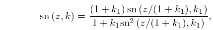
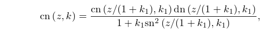
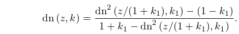
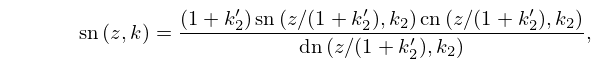
13: 22.7 Landen Transformations

… ►

22.7.2

\operatorname{sn}\left(z,k\right)=\frac{(1+k_{1})\operatorname{sn}\left(z/(1+k% _{1}),k_{1}\right)}{1+k_{1}{\operatorname{sn}}^{2}\left(z/(1+k_{1}),k_{1}% \right)},

ⓘ

Symbols:: $\operatorname{sn}\left(\NVar{z},\NVar{k}\right)$ : Jacobian elliptic function, $z$ : complex, $k$ : modulus and $k_{1}$ : change of variable
A&S Ref:: 16.12.2
Referenced by:: §22.20(iii)
Permalink:: http://dlmf.nist.gov/22.7.E2
Encodings:: pMML, png, TeX
See also:: Annotations for §22.7(i), §22.7 and Ch.22

►

22.7.3

\operatorname{cn}\left(z,k\right)=\frac{\operatorname{cn}\left(z/(1+k_{1}),k_{% 1}\right)\operatorname{dn}\left(z/(1+k_{1}),k_{1}\right)}{1+k_{1}{% \operatorname{sn}}^{2}\left(z/(1+k_{1}),k_{1}\right)},

ⓘ

Symbols:: $\operatorname{cn}\left(\NVar{z},\NVar{k}\right)$ : Jacobian elliptic function, $\operatorname{dn}\left(\NVar{z},\NVar{k}\right)$ : Jacobian elliptic function, $\operatorname{sn}\left(\NVar{z},\NVar{k}\right)$ : Jacobian elliptic function, $z$ : complex, $k$ : modulus and $k_{1}$ : change of variable
A&S Ref:: 16.12.3
Referenced by:: §22.20(iii)
Permalink:: http://dlmf.nist.gov/22.7.E3
Encodings:: pMML, png, TeX
See also:: Annotations for §22.7(i), §22.7 and Ch.22

►

22.7.4

\operatorname{dn}\left(z,k\right)=\frac{{\operatorname{dn}}^{2}\left(z/(1+k_{1% }),k_{1}\right)-(1-k_{1})}{1+k_{1}-{\operatorname{dn}}^{2}\left(z/(1+k_{1}),k_% {1}\right)}.

ⓘ

Symbols:: $\operatorname{dn}\left(\NVar{z},\NVar{k}\right)$ : Jacobian elliptic function, $z$ : complex, $k$ : modulus and $k_{1}$ : change of variable
A&S Ref:: 16.12.4
Referenced by:: §22.20(iii)
Permalink:: http://dlmf.nist.gov/22.7.E4
Encodings:: pMML, png, TeX
See also:: Annotations for §22.7(i), §22.7 and Ch.22

… ►

22.7.6

\operatorname{sn}\left(z,k\right)=\frac{(1+k_{2}^{\prime})\operatorname{sn}% \left(z/(1+k_{2}^{\prime}),k_{2}\right)\operatorname{cn}\left(z/(1+k_{2}^{% \prime}),k_{2}\right)}{\operatorname{dn}\left(z/(1+k_{2}^{\prime}),k_{2}\right% )},

ⓘ

Symbols:: $\operatorname{cn}\left(\NVar{z},\NVar{k}\right)$ : Jacobian elliptic function, $\operatorname{dn}\left(\NVar{z},\NVar{k}\right)$ : Jacobian elliptic function, $\operatorname{sn}\left(\NVar{z},\NVar{k}\right)$ : Jacobian elliptic function, $z$ : complex, $k$ : modulus, $k_{2}$ : change of variable and $k_{2}^{\prime}$ : change of variable
A&S Ref:: 16.14.2
Permalink:: http://dlmf.nist.gov/22.7.E6
Encodings:: pMML, png, TeX
See also:: Annotations for §22.7(ii), §22.7 and Ch.22

… ►

22.7.8

\operatorname{dn}\left(z,k\right)=\frac{(1-k_{2}^{\prime})({\operatorname{dn}}% ^{2}\left(z/(1+k_{2}^{\prime}),k_{2}\right)+k_{2}^{\prime})}{k_{2}^{2}% \operatorname{dn}\left(z/(1+k_{2}^{\prime}),k_{2}\right)}.

ⓘ

Symbols:: $\operatorname{dn}\left(\NVar{z},\NVar{k}\right)$ : Jacobian elliptic function, $z$ : complex, $k$ : modulus, $k_{2}$ : change of variable and $k_{2}^{\prime}$ : change of variable
A&S Ref:: 16.14.4
Permalink:: http://dlmf.nist.gov/22.7.E8
Encodings:: pMML, png, TeX
See also:: Annotations for §22.7(ii), §22.7 and Ch.22

…

14: 20.11 Generalizations and Analogs

… ►This is Jacobi’s inversion problem of §20.9(ii). … ►Each provides an extension of Jacobi’s inversion problem. … ►For

m=1,2,3,4

n=1,2,3,4

, and

m\neq n

, define twelve combined theta functions

\varphi_{m,n}\left(z,q\right)

by … ►

20.11.9

\varphi_{m,n}\left(z,q\right)=\varphi_{m,1}\left(z,q\right)\varphi_{1,n}\left(% z,q\right)=\frac{1}{\varphi_{n,m}\left(z,q\right)}=\frac{\varphi_{m,1}\left(z,% q\right)}{\varphi_{n,1}\left(z,q\right)}=\frac{\varphi_{1,n}\left(z,q\right)}{% \varphi_{1,m}\left(z,q\right)}.

ⓘ

Symbols:: $\varphi_{\NVar{n},\NVar{m}}\left(\NVar{z},\NVar{q}\right)$ : combined theta function, $m$ : integer, $n$ : integer, $z$ : complex and $q$ : nome
Permalink:: http://dlmf.nist.gov/20.11.E9
Encodings:: pMML, png, TeX
See also:: Annotations for §20.11(v), §20.11 and Ch.20

…

15: 18.14 Inequalities

… ►

Jacobi

… ►

Jacobi

… ►

Jacobi

… ►

Szegő–Szász Inequality

… ►

Jacobi

…

16: 27.9 Quadratic Characters

… ►

27.9.3

(p|q)(q|p)=(-1)^{(p-1)(q-1)/4}.

ⓘ

Symbols:: $(\NVar{n}|\NVar{p})$ : Legendre symbol, $p$ : odd prime and $q$ : odd prime
Referenced by:: §27.9
Permalink:: http://dlmf.nist.gov/27.9.E3
Encodings:: pMML, png, TeX
See also:: Annotations for §27.9 and Ch.27

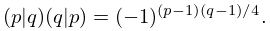
►If an odd integer

P

has prime factorization

P=\prod_{r=1}^{\nu\left(n\right)}p^{a_{r}}_{r}

, then the Jacobi symbol

(n|P)

is defined by

(n|P)=\prod_{r=1}^{\nu\left(n\right)}{(n|p_{r})}^{a_{r}}

, with

(n|1)=1

. The Jacobi symbol

(n|P)

is a Dirichlet character (mod

P

). …

17: 22.2 Definitions

… ►

22.2.4

\operatorname{sn}\left(z,k\right)=\frac{\theta_{3}\left(0,q\right)}{\theta_{2}% \left(0,q\right)}\frac{\theta_{1}\left(\zeta,q\right)}{\theta_{4}\left(\zeta,q% \right)}=\frac{1}{\operatorname{ns}\left(z,k\right)},

ⓘ

Defines:: $\operatorname{ns}\left(\NVar{z},\NVar{k}\right)$ : Jacobian elliptic function and $\operatorname{sn}\left(\NVar{z},\NVar{k}\right)$ : Jacobian elliptic function
Symbols:: $\theta_{\NVar{j}}\left(\NVar{z},\NVar{q}\right)$ : theta function, $q$ : nome, $z$ : complex, $k$ : modulus and $\zeta$ : change of variable
Referenced by:: §23.6(ii)
Permalink:: http://dlmf.nist.gov/22.2.E4
Encodings:: pMML, png, TeX
See also:: Annotations for §22.2 and Ch.22

►

22.2.5

\operatorname{cn}\left(z,k\right)=\frac{\theta_{4}\left(0,q\right)}{\theta_{2}% \left(0,q\right)}\frac{\theta_{2}\left(\zeta,q\right)}{\theta_{4}\left(\zeta,q% \right)}=\frac{1}{\operatorname{nc}\left(z,k\right)},

ⓘ

Defines:: $\operatorname{cn}\left(\NVar{z},\NVar{k}\right)$ : Jacobian elliptic function and $\operatorname{nc}\left(\NVar{z},\NVar{k}\right)$ : Jacobian elliptic function
Symbols:: $\theta_{\NVar{j}}\left(\NVar{z},\NVar{q}\right)$ : theta function, $q$ : nome, $z$ : complex, $k$ : modulus and $\zeta$ : change of variable
Permalink:: http://dlmf.nist.gov/22.2.E5
Encodings:: pMML, png, TeX
See also:: Annotations for §22.2 and Ch.22

►

22.2.6

\operatorname{dn}\left(z,k\right)=\frac{\theta_{4}\left(0,q\right)}{\theta_{3}% \left(0,q\right)}\frac{\theta_{3}\left(\zeta,q\right)}{\theta_{4}\left(\zeta,q% \right)}=\frac{1}{\operatorname{nd}\left(z,k\right)},

ⓘ

Defines:: $\operatorname{dn}\left(\NVar{z},\NVar{k}\right)$ : Jacobian elliptic function and $\operatorname{nd}\left(\NVar{z},\NVar{k}\right)$ : Jacobian elliptic function
Symbols:: $\theta_{\NVar{j}}\left(\NVar{z},\NVar{q}\right)$ : theta function, $q$ : nome, $z$ : complex, $k$ : modulus and $\zeta$ : change of variable
Referenced by:: §22.20(ii)
Permalink:: http://dlmf.nist.gov/22.2.E6
Encodings:: pMML, png, TeX
See also:: Annotations for §22.2 and Ch.22

►

22.2.7

\operatorname{sd}\left(z,k\right)=\frac{{\theta_{3}}^{2}\left(0,q\right)}{% \theta_{2}\left(0,q\right)\theta_{4}\left(0,q\right)}\frac{\theta_{1}\left(% \zeta,q\right)}{\theta_{3}\left(\zeta,q\right)}=\frac{1}{\operatorname{ds}% \left(z,k\right)},

ⓘ

Defines:: $\operatorname{ds}\left(\NVar{z},\NVar{k}\right)$ : Jacobian elliptic function and $\operatorname{sd}\left(\NVar{z},\NVar{k}\right)$ : Jacobian elliptic function
Symbols:: $\theta_{\NVar{j}}\left(\NVar{z},\NVar{q}\right)$ : theta function, $q$ : nome, $z$ : complex, $k$ : modulus and $\zeta$ : change of variable
Permalink:: http://dlmf.nist.gov/22.2.E7
Encodings:: pMML, png, TeX
See also:: Annotations for §22.2 and Ch.22

… ►

\operatorname{ss}\left(z,k\right)=1

. …

18: 18.6 Symmetry, Special Values, and Limits to Monomials

… ►For Jacobi, ultraspherical, Chebyshev, Legendre, and Hermite polynomials, see Table 18.6.1. … ►

Table 18.6.1: Classical OP’s: symmetry and special values.

► ►►

$p_{n}(x)$	$p_{n}(-x)$	$p_{n}(1)$	$p_{2n}(0)$	$p_{2n+1}^{\prime}(0)$
…

► ►

§18.6(ii) Limits to Monomials

►

18.6.2

\lim_{\alpha\to\infty}\frac{P^{(\alpha,\beta)}_{n}\left(x\right)}{P^{(\alpha,% \beta)}_{n}\left(1\right)}=\left(\frac{1+x}{2}\right)^{n},

ⓘ

Symbols:: $P^{(\NVar{\alpha},\NVar{\beta})}_{\NVar{n}}\left(\NVar{x}\right)$ : Jacobi polynomial, $n$ : nonnegative integer and $x$ : real variable
Referenced by:: §18.6(ii)
Permalink:: http://dlmf.nist.gov/18.6.E2
Encodings:: pMML, png, TeX
See also:: Annotations for §18.6(ii), §18.6 and Ch.18

►

18.6.3

\lim_{\beta\to\infty}\frac{P^{(\alpha,\beta)}_{n}\left(x\right)}{P^{(\alpha,% \beta)}_{n}\left(-1\right)}=\left(\frac{1-x}{2}\right)^{n},

ⓘ

Symbols:: $P^{(\NVar{\alpha},\NVar{\beta})}_{\NVar{n}}\left(\NVar{x}\right)$ : Jacobi polynomial, $n$ : nonnegative integer and $x$ : real variable
Referenced by:: §18.6(ii)
Permalink:: http://dlmf.nist.gov/18.6.E3
Encodings:: pMML, png, TeX
See also:: Annotations for §18.6(ii), §18.6 and Ch.18

…

19: 20.15 Tables

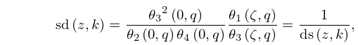
… ►This reference gives

\theta_{j}\left(x,q\right)

j=1,2,3,4

, and their logarithmic

x

-derivatives to 4D for

x/\pi=0(.1)1

\alpha=0(9^{\circ})90^{\circ}

, where

\alpha

is the modular angle given by ►

20.15.1

\sin\alpha={\theta_{2}}^{2}\left(0,q\right)/{\theta_{3}}^{2}\left(0,q\right)=k.

ⓘ

Defines:: $\alpha$ : modular angle (locally)
Symbols:: $\theta_{\NVar{j}}\left(\NVar{z},\NVar{q}\right)$ : theta function, $\sin\NVar{z}$ : sine function and $q$ : nome
Referenced by:: §20.15, §20.15
Permalink:: http://dlmf.nist.gov/20.15.E1
Encodings:: pMML, png, TeX
See also:: Annotations for §20.15 and Ch.20

►Spenceley and Spenceley (1947) tabulates

\theta_{1}\left(x,q\right)/\theta_{2}\left(0,q\right)

\theta_{2}\left(x,q\right)/\theta_{2}\left(0,q\right)

\theta_{3}\left(x,q\right)/\theta_{4}\left(0,q\right)

\theta_{4}\left(x,q\right)/\theta_{4}\left(0,q\right)

to 12D for

u=0(1^{\circ})90^{\circ}

\alpha=0(1^{\circ})89^{\circ}

, where

u=2x/(\pi{\theta_{3}}^{2}\left(0,q\right))

and

\alpha

is defined by (20.15.1), together with the corresponding values of

\theta_{2}\left(0,q\right)

and

\theta_{4}\left(0,q\right)

. ►Lawden (1989, pp. 270–279) tabulates

\theta_{j}\left(x,q\right)

j=1,2,3,4

, to 5D for

x=0(1^{\circ})90^{\circ}

q=0.1(.1)0.9

, and also

q

to 5D for

k^{2}=0(.01)1

. ►Tables of Neville’s theta functions

\theta_{s}\left(x,q\right)

\theta_{c}\left(x,q\right)

\theta_{d}\left(x,q\right)

\theta_{n}\left(x,q\right)

(see §20.1) and their logarithmic

x

-derivatives are given in Abramowitz and Stegun (1964, pp. 582–585) to 9D for

\varepsilon,\alpha=0(5^{\circ})90^{\circ}

, where (in radian measure)

\varepsilon=x/{\theta_{3}}^{2}\left(0,q\right)=\pi x/(2K\left(k\right))

, and

\alpha

is defined by (20.15.1). …

20: 20.8 Watson’s Expansions

… ►

20.8.1

\frac{\theta_{2}\left(0,q\right)\theta_{3}\left(z,q\right)\theta_{4}\left(z,q% \right)}{\theta_{2}\left(z,q\right)}=2\sum_{n=-\infty}^{\infty}\frac{(-1)^{n}q% ^{n^{2}}e^{i2nz}}{q^{-n}e^{-iz}+q^{n}e^{iz}}.

ⓘ

Symbols:: $\theta_{\NVar{j}}\left(\NVar{z},\NVar{q}\right)$ : theta function, $\mathrm{e}$ : base of natural logarithm, $\mathrm{i}$ : imaginary unit, $n$ : integer, $z$ : complex and $q$ : nome
Permalink:: http://dlmf.nist.gov/20.8.E1
Encodings:: pMML, png, TeX
See also:: Annotations for §20.8 and Ch.20

…

Jacobi

11—20 of 126 matching pages

11: 18.7 Interrelations and Limit Relations

Ultraspherical and Jacobi

Chebyshev, Ultraspherical, and Jacobi

Legendre, Ultraspherical, and Jacobi

Jacobi → Laguerre

Jacobi → Hermite

12: 22.14 Integrals

13: 22.7 Landen Transformations

14: 20.11 Generalizations and Analogs

15: 18.14 Inequalities

Jacobi

Jacobi

Jacobi

Szegő–Szász Inequality

Jacobi

16: 27.9 Quadratic Characters

17: 22.2 Definitions

18: 18.6 Symmetry, Special Values, and Limits to Monomials

§18.6(ii) Limits to Monomials

19: 20.15 Tables

20: 20.8 Watson’s Expansions

Jacobi $\to$ Laguerre

Jacobi $\to$ Hermite