Jacobi%E2%80%99s

(0.009 seconds)

1—10 of 622 matching pages

►The classical OP’s comprise the Jacobi, Laguerre and Hermite polynomials. … ►This table also includes the following special cases of Jacobi polynomials: ultraspherical, Chebyshev, and Legendre. … ►For finite power series of the Jacobi, ultraspherical, Laguerre, and Hermite polynomials, see §18.5(iii) (in powers of

x-1

for Jacobi polynomials, in powers of

x

for the other cases). … ►

Jacobi on Other Intervals

…

3: 31.2 Differential Equations

… ►

§31.2(i) Heun’s Equation

… ►

Jacobi’s Elliptic Form

… ►

Weierstrass’s Form

… ►

§31.2(v) Heun’s Equation Automorphisms

… ►

Composite Transformations

…

4: 29.2 Differential Equations

… ►

§29.2(i) Lamé’s Equation

… ►For

\operatorname{sn}\left(z,k\right)

see §22.2. … ►

§29.2(ii) Other Forms

… ►For

\operatorname{am}\left(z,k\right)

see §22.16(i). … ►

5: 7.20 Mathematical Applications

… ►

§7.20(ii) Cornu’s Spiral

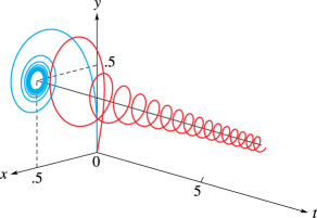
►Let the set

\{x(t),y(t),t\}

be defined by

x(t)=C\left(t\right)

y(t)=S\left(t\right)

t\geq 0

. Then the set

\{x(t),y(t)\}

is called Cornu’s spiral: it is the projection of the corkscrew on the

\{x,y\}

-plane. … ►

See accompanying text — Figure 7.20.1: Cornu’s spiral, formed from Fresnel integrals, is defined parametrically by $x=C\left(t\right)$ , $y=S\left(t\right)$ , $t\in[0,\infty)$ . Magnify

…

6: 28.2 Definitions and Basic Properties

… ►

§28.2(i) Mathieu’s Equation

… ►

§28.2(iii) Floquet’s Theorem and the Characteristic Exponents

… ►This is the characteristic equation of Mathieu’s equation (28.2.1). … ►

§28.2(iv) Floquet Solutions

… ► …

7: 7.2 Definitions

… ►

§7.2(ii) Dawson’s Integral

►

7.2.5

F\left(z\right)=e^{-z^{2}}\int_{0}^{z}e^{t^{2}}\,\mathrm{d}t.

ⓘ

Defines:: $F\left(\NVar{z}\right)$ : Dawson’s integral
Symbols:: $\,\mathrm{d}\NVar{x}$ : differential of $x$ , $\mathrm{e}$ : base of natural logarithm, $\int$ : integral and $z$ : complex variable
A&S Ref:: 7.1.1
Permalink:: http://dlmf.nist.gov/7.2.E5
Encodings:: pMML, png, TeX
See also:: Annotations for §7.2(ii), §7.2 and Ch.7

… ►

7.2.8

S\left(z\right)=\int_{0}^{z}\sin\left(\tfrac{1}{2}\pi t^{2}\right)\,\mathrm{d}t,

ⓘ

Defines:: $S\left(\NVar{z}\right)$ : Fresnel integral
Symbols:: $\pi$ : the ratio of the circumference of a circle to its diameter, $\,\mathrm{d}\NVar{x}$ : differential of $x$ , $\int$ : integral, $\sin\NVar{z}$ : sine function and $z$ : complex variable
A&S Ref:: 7.3.2
Referenced by:: §7.5, §7.6(i)
Permalink:: http://dlmf.nist.gov/7.2.E8
Encodings:: pMML, png, TeX
See also:: Annotations for §7.2(iii), §7.2 and Ch.7

►

\mathcal{F}\left(z\right)

C\left(z\right)

, and

S\left(z\right)

are entire functions of

z

, as are

\mathrm{f}\left(z\right)

and

\mathrm{g}\left(z\right)

in the next subsection. … ►

\lim_{x\to\infty}S\left(x\right)=\tfrac{1}{2}.

…

8: 28.20 Definitions and Basic Properties

… ►

§28.20(i) Modified Mathieu’s Equation

►When

z

is replaced by

\pm\mathrm{i}z

, (28.2.1) becomes the modified Mathieu’s equation: ►

28.20.1

w^{\prime\prime}-\left(a-2q\cosh\left(2z\right)\right)w=0,

ⓘ

Symbols:: $\cosh\NVar{z}$ : hyperbolic cosine function, $q=h^{2}$ : parameter, $z$ : complex variable, $a$ : parameter and $w(z)$ : Mathieu’s equation solution
A&S Ref:: 20.1.2 (in slightly different form) 20.8.6
Referenced by:: §28.20(iii), §28.32(i), 1st item, 2nd item, item (b), §28.8(iv), §28.8(iv)
Permalink:: http://dlmf.nist.gov/28.20.E1
Encodings:: pMML, png, TeX
See also:: Annotations for §28.20(i), §28.20 and Ch.28

… ►

28.20.2

{(\zeta^{2}-1)w^{\prime\prime}+\zeta w^{\prime}+\left(4q\zeta^{2}-2q-a\right)w% =0},

\zeta=\cosh z

ⓘ

Symbols:: $\cosh\NVar{z}$ : hyperbolic cosine function, $q=h^{2}$ : parameter, $z$ : complex variable, $a$ : parameter and $w(z)$ : Mathieu’s equation solution
Referenced by:: §28.20(iii)
Permalink:: http://dlmf.nist.gov/28.20.E2
Encodings:: pMML, png, TeX
See also:: Annotations for §28.20(i), §28.20 and Ch.28

… ►For

s\in\mathbb{Z}

, …

9: 22.8 Addition Theorems

… ►

22.8.14

\operatorname{sn}(u+v)=\frac{\operatorname{sn}u\operatorname{cn}u\operatorname% {dn}v+\operatorname{sn}v\operatorname{cn}v\operatorname{dn}u}{\operatorname{cn% }u\operatorname{cn}v+\operatorname{sn}u\operatorname{dn}u\operatorname{sn}v% \operatorname{dn}v},

ⓘ

Symbols:: $\operatorname{cn}\left(\NVar{z},\NVar{k}\right)$ : Jacobian elliptic function, $\operatorname{dn}\left(\NVar{z},\NVar{k}\right)$ : Jacobian elliptic function, $\operatorname{sn}\left(\NVar{z},\NVar{k}\right)$ : Jacobian elliptic function, $u$ : complex, $v$ : complex and $k$ : modulus
Permalink:: http://dlmf.nist.gov/22.8.E14
Encodings:: pMML, png, TeX
See also:: Annotations for §22.8(ii), §22.8 and Ch.22

►

22.8.15

\operatorname{cn}(u+v)=\frac{\operatorname{sn}u\operatorname{cn}u\operatorname% {dn}v-\operatorname{sn}v\operatorname{cn}v\operatorname{dn}u}{\operatorname{sn% }u\operatorname{cn}v\operatorname{dn}v-\operatorname{sn}v\operatorname{cn}u% \operatorname{dn}u},

ⓘ

Symbols:: $\operatorname{cn}\left(\NVar{z},\NVar{k}\right)$ : Jacobian elliptic function, $\operatorname{dn}\left(\NVar{z},\NVar{k}\right)$ : Jacobian elliptic function, $\operatorname{sn}\left(\NVar{z},\NVar{k}\right)$ : Jacobian elliptic function, $u$ : complex, $v$ : complex and $k$ : modulus
Permalink:: http://dlmf.nist.gov/22.8.E15
Encodings:: pMML, png, TeX
See also:: Annotations for §22.8(ii), §22.8 and Ch.22

… ►

22.8.17

\operatorname{dn}(u+v)=\frac{\operatorname{sn}u\operatorname{cn}v\operatorname% {dn}u-\operatorname{sn}v\operatorname{cn}u\operatorname{dn}v}{\operatorname{sn% }u\operatorname{cn}v\operatorname{dn}v-\operatorname{sn}v\operatorname{cn}u% \operatorname{dn}u},

ⓘ

Symbols:: $\operatorname{cn}\left(\NVar{z},\NVar{k}\right)$ : Jacobian elliptic function, $\operatorname{dn}\left(\NVar{z},\NVar{k}\right)$ : Jacobian elliptic function, $\operatorname{sn}\left(\NVar{z},\NVar{k}\right)$ : Jacobian elliptic function, $u$ : complex, $v$ : complex and $k$ : modulus
Permalink:: http://dlmf.nist.gov/22.8.E17
Encodings:: pMML, png, TeX
See also:: Annotations for §22.8(ii), §22.8 and Ch.22

… ►

22.8.23

\begin{vmatrix}\operatorname{sn}z_{1}\operatorname{cn}z_{1}&\operatorname{cn}z% _{1}\operatorname{dn}z_{1}&\operatorname{cn}z_{1}&\operatorname{dn}z_{1}\\ \operatorname{sn}z_{2}\operatorname{cn}z_{2}&\operatorname{cn}z_{2}% \operatorname{dn}z_{2}&\operatorname{cn}z_{2}&\operatorname{dn}z_{2}\\ \operatorname{sn}z_{3}\operatorname{cn}z_{3}&\operatorname{cn}z_{3}% \operatorname{dn}z_{3}&\operatorname{cn}z_{3}&\operatorname{dn}z_{3}\\ \operatorname{sn}z_{4}\operatorname{cn}z_{4}&\operatorname{cn}z_{4}% \operatorname{dn}z_{4}&\operatorname{cn}z_{4}&\operatorname{dn}z_{4}\end{% vmatrix}=0.

ⓘ

Symbols:: $\operatorname{cn}\left(\NVar{z},\NVar{k}\right)$ : Jacobian elliptic function, $\operatorname{dn}\left(\NVar{z},\NVar{k}\right)$ : Jacobian elliptic function, $\operatorname{sn}\left(\NVar{z},\NVar{k}\right)$ : Jacobian elliptic function, $\det$ : determinant, $z$ : complex and $k$ : modulus
Permalink:: http://dlmf.nist.gov/22.8.E23
Encodings:: pMML, png, TeX
See also:: Annotations for §22.8(iii), §22.8 and Ch.22

… ►If sums/differences of the

z_{j}

’s are rational multiples of

K\left(k\right)

, then further relations follow. …

10: 22.6 Elementary Identities

… ►

22.6.2

1+{\operatorname{cs}}^{2}\left(z,k\right)=k^{2}+{\operatorname{ds}}^{2}\left(z% ,k\right)={\operatorname{ns}}^{2}\left(z,k\right),

ⓘ

Symbols:: $\operatorname{cs}\left(\NVar{z},\NVar{k}\right)$ : Jacobian elliptic function, $\operatorname{ds}\left(\NVar{z},\NVar{k}\right)$ : Jacobian elliptic function, $\operatorname{ns}\left(\NVar{z},\NVar{k}\right)$ : Jacobian elliptic function, $z$ : complex and $k$ : modulus
A&S Ref:: 16.9.4
Permalink:: http://dlmf.nist.gov/22.6.E2
Encodings:: pMML, png, TeX
See also:: Annotations for §22.6(i), §22.6 and Ch.22

… ►

22.6.5

\operatorname{sn}\left(2z,k\right)=\frac{2\operatorname{sn}\left(z,k\right)% \operatorname{cn}\left(z,k\right)\operatorname{dn}\left(z,k\right)}{1-k^{2}{% \operatorname{sn}}^{4}\left(z,k\right)},

ⓘ

Symbols:: $\operatorname{cn}\left(\NVar{z},\NVar{k}\right)$ : Jacobian elliptic function, $\operatorname{dn}\left(\NVar{z},\NVar{k}\right)$ : Jacobian elliptic function, $\operatorname{sn}\left(\NVar{z},\NVar{k}\right)$ : Jacobian elliptic function, $z$ : complex and $k$ : modulus
A&S Ref:: 16.18.1
Permalink:: http://dlmf.nist.gov/22.6.E5
Encodings:: pMML, png, TeX
See also:: Annotations for §22.6(ii), §22.6 and Ch.22

… ►

22.6.22

{\operatorname{pq}}^{2}\left(\tfrac{1}{2}z,k\right)=\frac{\operatorname{ps}% \left(z,k\right)+\operatorname{rs}\left(z,k\right)}{\operatorname{qs}\left(z,k% \right)+\operatorname{rs}\left(z,k\right)}=\frac{\operatorname{pq}\left(z,k% \right)+\operatorname{rq}\left(z,k\right)}{1+\operatorname{rq}\left(z,k\right)% }=\frac{\operatorname{pr}\left(z,k\right)+1}{\operatorname{qr}\left(z,k\right)% +1}.

ⓘ

Symbols:: $\operatorname{pq}\left(\NVar{z},\NVar{k}\right)$ : generic Jacobian elliptic function, $z$ : complex and $k$ : modulus
Referenced by:: §22.6(iii)
Permalink:: http://dlmf.nist.gov/22.6.E22
Encodings:: pMML, png, TeX
See also:: Annotations for §22.6(iii), §22.6 and Ch.22

… ►

§22.6(iv) Rotation of Argument (Jacobi’s Imaginary Transformation)

►

Table 22.6.1: Jacobi’s imaginary transformation of Jacobian elliptic functions.

► ►►

$\operatorname{sn}\left(iz,k\right)$ $\;=\;$	$i\operatorname{sc}\left(z,k^{\prime}\right)$	$\operatorname{dc}\left(iz,k\right)$ $\;=\;$	$\operatorname{dn}\left(z,k^{\prime}\right)$
…

► …

Jacobi%E2%80%99s

1—10 of 622 matching pages

1: 22.16 Related Functions

§22.16(i) Jacobi’s Amplitude ( $\operatorname{am}$ ) Function

§22.16(ii) Jacobi’s Epsilon Function

Integral Representations

§22.16(iii) Jacobi’s Zeta Function

Definition

2: 18.3 Definitions

§18.3 Definitions

Jacobi on Other Intervals

3: 31.2 Differential Equations

§31.2(i) Heun’s Equation

Jacobi’s Elliptic Form

Weierstrass’s Form

§31.2(v) Heun’s Equation Automorphisms

Composite Transformations

4: 29.2 Differential Equations

§29.2(i) Lamé’s Equation

§29.2(ii) Other Forms

5: 7.20 Mathematical Applications

§7.20(ii) Cornu’s Spiral

6: 28.2 Definitions and Basic Properties

§28.2(i) Mathieu’s Equation

§28.2(iii) Floquet’s Theorem and the Characteristic Exponents

§28.2(iv) Floquet Solutions

7: 7.2 Definitions

§7.2(ii) Dawson’s Integral

8: 28.20 Definitions and Basic Properties

§28.20(i) Modified Mathieu’s Equation

9: 22.8 Addition Theorems

10: 22.6 Elementary Identities

§22.6(iv) Rotation of Argument (Jacobi’s Imaginary Transformation)

Jacobi%E2%80%99s

1—10 of 622 matching pages

1: 22.16 Related Functions

§22.16(i) Jacobi’s Amplitude ( am ) Function

§22.16(ii) Jacobi’s Epsilon Function

Integral Representations

§22.16(iii) Jacobi’s Zeta Function

Definition

2: 18.3 Definitions

§18.3 Definitions

Jacobi on Other Intervals

3: 31.2 Differential Equations

§31.2(i) Heun’s Equation

Jacobi’s Elliptic Form

Weierstrass’s Form

§31.2(v) Heun’s Equation Automorphisms

Composite Transformations

4: 29.2 Differential Equations

§29.2(i) Lamé’s Equation

§29.2(ii) Other Forms

5: 7.20 Mathematical Applications

§7.20(ii) Cornu’s Spiral

6: 28.2 Definitions and Basic Properties

§28.2(i) Mathieu’s Equation

§28.2(iii) Floquet’s Theorem and the Characteristic Exponents

§28.2(iv) Floquet Solutions

7: 7.2 Definitions

§7.2(ii) Dawson’s Integral

8: 28.20 Definitions and Basic Properties

§28.20(i) Modified Mathieu’s Equation

9: 22.8 Addition Theorems

10: 22.6 Elementary Identities

§22.6(iv) Rotation of Argument (Jacobi’s Imaginary Transformation)

§22.16(i) Jacobi’s Amplitude ( $\operatorname{am}$ ) Function