Jacobi zeta function

SearchAdvancedHelp

(0.008 seconds)

1—10 of 33 matching pages

1: 22.16 Related Functions

… ►

§22.16(iii) Jacobi’s Zeta Function

►

Definition

… ►

Properties

… ►

►►

Figure 22.16.3: Jacobi’s zeta function $\mathrm{Z}\left(x|k\right)$ for $0\le x\le 10\pi$ and $k=0.4,0.7,0.99,0.999999$. Magnify

2: 25.1 Special Notation

… ►The main related functions are the Hurwitz zeta function $\zeta (s,a)$, the dilogarithm ${\mathrm{Li}}_2\left(z\right)$, the polylogarithm ${\mathrm{Li}}_s\left(z\right)$ (also known as Jonquière’s function $\varphi (z,s)$), Lerch’s transcendent $\mathrm{\Phi }(z,s,a)$, and the Dirichlet $L$-functions $L(s,\chi )$.

3: 22.21 Tables

… ► …

4: 22.1 Special Notation

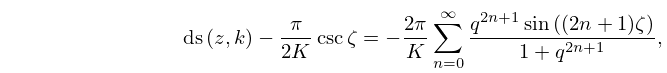
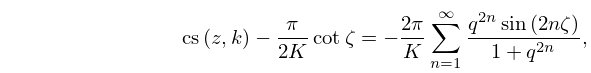
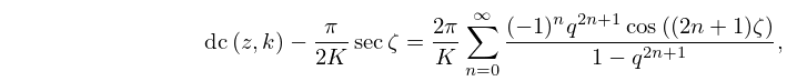
… ►The functions treated in this chapter are the three principal Jacobian elliptic functions $\mathrm{sn}(z,k)$, $\mathrm{cn}(z,k)$, $\mathrm{dn}(z,k)$; the nine subsidiary Jacobian elliptic functions $\mathrm{cd}(z,k)$, $\mathrm{sd}(z,k)$, $\mathrm{nd}(z,k)$, $\mathrm{dc}(z,k)$, $\mathrm{nc}(z,k)$, $\mathrm{sc}(z,k)$, $\mathrm{ns}(z,k)$, $\mathrm{ds}(z,k)$, $\mathrm{cs}(z,k)$; the amplitude function $\mathrm{am}(x,k)$; Jacobi’s epsilon and zeta functions $ℰ(x,k)$ and $\mathrm{Z}\left(x|k\right)$. …

5: 22.20 Methods of Computation

… ►Jacobi’s zeta function can then be found by use of (22.16.32). …

6: 27.1 Special Notation

… ►(For other notation see Notation for the Special Functions.) ► ►►►►

$d,k,m,n$	positive integers (unless otherwise indicated).
…
$\zeta \left(s\right)$	Riemann zeta function; see §25.2(i).
$(n|P)$	Jacobi symbol; see §27.9.
…

7: 20.10 Integrals

… ►

20.10.1 $${\int }_0^{\mathrm{\infty }}{x}^{s-1}{\theta }_2\left(0\right|\mathrm{i}{x}^2)dx=2^s(1-2^{-s}){\pi }^{-s/2}\mathrm{\Gamma }\left(\frac{1}{2}s\right)\zeta \left(s\right),$$ $\mathrm{\Re }s>1$,

ⓘ

Symbols:

$\mathrm{\Gamma }\left(z\right)$: gamma function, ${\theta }_j\left(z\right|\tau )$: theta function, $\zeta \left(s\right)$: Riemann zeta function, $\pi$: the ratio of the circumference of a circle to its diameter, $dx$: differential of $x$ , $\mathrm{i}$: imaginary unit, $\int$: integral and $\mathrm{\Re }$: real part

Keywords:

Mellin transform

Referenced by:

§20.10(i), Erratum (V1.1.5) for §20.10(i)

Permalink:

http://dlmf.nist.gov/20.10.E1

Encodings:

pMML, png, TeX

Modification (effective with 1.1.5):

Originally the constraint was $\mathrm{\Re }s>2$. This can be relaxed to $\mathrm{\Re }s>1$ because ${\theta }_2\left(0\right|\mathrm{i}{x}^2)=x^{-1}{\theta }_4\left(0\right|\mathrm{i}{x}^{-2})\sim x^{-1}$ as $x\to 0+$, which follows from (20.7.31) and (20.4.5).

See also:

Annotations for §20.10(i), §20.10 and Ch.20

►

20.10.2 $${\int }_0^{\mathrm{\infty }}{x}^{s-1}({\theta }_3\left(0\right|\mathrm{i}{x}^2)-1)dx={\pi }^{-s/2}\mathrm{\Gamma }\left(\frac{1}{2}s\right)\zeta \left(s\right),$$ $\mathrm{\Re }s>1$,

ⓘ

Symbols:

$\mathrm{\Gamma }\left(z\right)$: gamma function, ${\theta }_j\left(z\right|\tau )$: theta function, $\zeta \left(s\right)$: Riemann zeta function, $\pi$: the ratio of the circumference of a circle to its diameter, $dx$: differential of $x$ , $\mathrm{i}$: imaginary unit, $\int$: integral and $\mathrm{\Re }$: real part

Keywords:

Mellin transform

Referenced by:

§20.10(i), Erratum (V1.1.5) for §20.10(i)

Permalink:

http://dlmf.nist.gov/20.10.E2

Encodings:

pMML, png, TeX

Modification (effective with 1.1.5):

Originally the constraint was $\mathrm{\Re }s>2$. This can be relaxed to $\mathrm{\Re }s>1$ because ${\theta }_3\left(0\right|\mathrm{i}{x}^2)=x^{-1}{\theta }_3\left(0\right|\mathrm{i}{x}^{-2})\sim x^{-1}$ as $x\to 0+$, which follows from (20.7.32) and (20.4.4).

See also:

Annotations for §20.10(i), §20.10 and Ch.20

►

20.10.3 $${\int }_0^{\mathrm{\infty }}{x}^{s-1}(1-{\theta }_4\left(0\right|\mathrm{i}{x}^2))dx=(1-2^{1-s}){\pi }^{-s/2}\mathrm{\Gamma }\left(\frac{1}{2}s\right)\zeta \left(s\right),$$ $\mathrm{\Re }s>0$.

ⓘ

Symbols:

$\mathrm{\Gamma }\left(z\right)$: gamma function, ${\theta }_j\left(z\right|\tau )$: theta function, $\zeta \left(s\right)$: Riemann zeta function, $\pi$: the ratio of the circumference of a circle to its diameter, $dx$: differential of $x$ , $\mathrm{i}$: imaginary unit, $\int$: integral and $\mathrm{\Re }$: real part

Keywords:

Mellin transform

Referenced by:

§20.10(i), Erratum (V1.1.5) for §20.10(i)

Permalink:

http://dlmf.nist.gov/20.10.E3

Encodings:

pMML, png, TeX

Modification (effective with 1.1.5):

Originally the constraint was $\mathrm{\Re }s>2$. This can be relaxed to $\mathrm{\Re }s>0$ because $1-{\theta }_4\left(0\right|\mathrm{i}{x}^2)=1-x^{-1}{\theta }_2\left(0\right|\mathrm{i}{x}^{-2})\sim 1$ as $x\to 0+$, which follows from (20.7.33) and (20.4.3).

See also:

Annotations for §20.10(i), §20.10 and Ch.20

…

8: 31.7 Relations to Other Functions

§31.7 Relations to Other Functions

►

§31.7(i) Reductions to the Gauss Hypergeometric Function

… ►

§31.7(ii) Relations to Lamé Functions

►With $z={\mathrm{sn}}^2(\zeta ,k)$ and …equation (31.2.1) becomes Lamé’s equation with independent variable $\zeta$; compare (29.2.1) and (31.2.8). …

9: 22.2 Definitions

… ►

22.2.4 $$\mathrm{sn}(z,k)=\frac{{\theta }_3(0,q)}{{\theta }_2(0,q)}\frac{{\theta }_1(\zeta ,q)}{{\theta }_4(\zeta ,q)}=\frac{1}{\mathrm{ns}(z,k)},$$

ⓘ

Defines:

$\mathrm{ns}(z,k)$: Jacobian elliptic function and $\mathrm{sn}(z,k)$: Jacobian elliptic function

Symbols:

${\theta }_j(z,q)$: theta function, $q$: nome, $z$: complex, $k$: modulus and $\zeta$: change of variable

Referenced by:

§23.6(ii)

Permalink:

http://dlmf.nist.gov/22.2.E4

Encodings:

pMML, png, TeX

See also:

Annotations for §22.2 and Ch.22

►

22.2.5 $$\mathrm{cn}(z,k)=\frac{{\theta }_4(0,q)}{{\theta }_2(0,q)}\frac{{\theta }_2(\zeta ,q)}{{\theta }_4(\zeta ,q)}=\frac{1}{\mathrm{nc}(z,k)},$$

ⓘ

Defines:

$\mathrm{cn}(z,k)$: Jacobian elliptic function and $\mathrm{nc}(z,k)$: Jacobian elliptic function

Symbols:

${\theta }_j(z,q)$: theta function, $q$: nome, $z$: complex, $k$: modulus and $\zeta$: change of variable

Permalink:

http://dlmf.nist.gov/22.2.E5

Encodings:

pMML, png, TeX

See also:

Annotations for §22.2 and Ch.22

►

22.2.6 $$\mathrm{dn}(z,k)=\frac{{\theta }_4(0,q)}{{\theta }_3(0,q)}\frac{{\theta }_3(\zeta ,q)}{{\theta }_4(\zeta ,q)}=\frac{1}{\mathrm{nd}(z,k)},$$

ⓘ

Defines:

$\mathrm{dn}(z,k)$: Jacobian elliptic function and $\mathrm{nd}(z,k)$: Jacobian elliptic function

Symbols:

${\theta }_j(z,q)$: theta function, $q$: nome, $z$: complex, $k$: modulus and $\zeta$: change of variable

Referenced by:

§22.20(ii)

Permalink:

http://dlmf.nist.gov/22.2.E6

Encodings:

pMML, png, TeX

See also:

Annotations for §22.2 and Ch.22

►

22.2.7 $$\mathrm{sd}(z,k)=\frac{{\theta }_3^2(0,q)}{{\theta }_2(0,q){\theta }_4(0,q)}\frac{{\theta }_1(\zeta ,q)}{{\theta }_3(\zeta ,q)}=\frac{1}{\mathrm{ds}(z,k)},$$

ⓘ

Defines:

$\mathrm{ds}(z,k)$: Jacobian elliptic function and $\mathrm{sd}(z,k)$: Jacobian elliptic function

Symbols:

${\theta }_j(z,q)$: theta function, $q$: nome, $z$: complex, $k$: modulus and $\zeta$: change of variable

Permalink:

http://dlmf.nist.gov/22.2.E7

Encodings:

pMML, png, TeX

See also:

Annotations for §22.2 and Ch.22

►

22.2.8 $$\mathrm{cd}(z,k)=\frac{{\theta }_3(0,q)}{{\theta }_2(0,q)}\frac{{\theta }_2(\zeta ,q)}{{\theta }_3(\zeta ,q)}=\frac{1}{\mathrm{dc}(z,k)},$$

ⓘ

Defines:

$\mathrm{cd}(z,k)$: Jacobian elliptic function and $\mathrm{dc}(z,k)$: Jacobian elliptic function

Symbols:

${\theta }_j(z,q)$: theta function, $q$: nome, $z$: complex, $k$: modulus and $\zeta$: change of variable

Permalink:

http://dlmf.nist.gov/22.2.E8

Encodings:

pMML, png, TeX

See also:

Annotations for §22.2 and Ch.22

…

10: 22.11 Fourier and Hyperbolic Series

… ►

22.11.1 $$\mathrm{sn}(z,k)=\frac{2\pi }{Kk}\sum _{n=0}^{\mathrm{\infty }}\frac{q^{n+\frac{1}{2}}\sin \left((2n+1)\zeta \right)}{1-q^{2n+1}},$$

ⓘ

Symbols:

$\mathrm{sn}(z,k)$: Jacobian elliptic function, $\pi$: the ratio of the circumference of a circle to its diameter, $K\left(k\right)$: Legendre’s complete elliptic integral of the first kind, $q$: nome, $\sin z$: sine function, $z$: complex, $k$: modulus and $\zeta$: change of variable

A&S Ref:

16.23.1

Permalink:

http://dlmf.nist.gov/22.11.E1

Encodings:

pMML, png, TeX

See also:

Annotations for §22.11 and Ch.22

… ►

22.11.7 $$\mathrm{ns}(z,k)-\frac{\pi }{2K}\csc \zeta =\frac{2\pi }{K}\sum _{n=0}^{\mathrm{\infty }}\frac{q^{2n+1}\sin \left((2n+1)\zeta \right)}{1-q^{2n+1}},$$

ⓘ

Symbols:

$\mathrm{ns}(z,k)$: Jacobian elliptic function, $\pi$: the ratio of the circumference of a circle to its diameter, $K\left(k\right)$: Legendre’s complete elliptic integral of the first kind, $\csc z$: cosecant function, $q$: nome, $\sin z$: sine function, $z$: complex, $k$: modulus and $\zeta$: change of variable

A&S Ref:

16.23.10

Referenced by:

§22.11

Permalink:

http://dlmf.nist.gov/22.11.E7

Encodings:

pMML, png, TeX

See also:

Annotations for §22.11 and Ch.22

►

22.11.8 $$\mathrm{ds}(z,k)-\frac{\pi }{2K}\csc \zeta =-\frac{2\pi }{K}\sum _{n=0}^{\mathrm{\infty }}\frac{q^{2n+1}\sin \left((2n+1)\zeta \right)}{1+q^{2n+1}},$$

ⓘ

Symbols:

$\mathrm{ds}(z,k)$: Jacobian elliptic function, $\pi$: the ratio of the circumference of a circle to its diameter, $K\left(k\right)$: Legendre’s complete elliptic integral of the first kind, $\csc z$: cosecant function, $q$: nome, $\sin z$: sine function, $z$: complex, $k$: modulus and $\zeta$: change of variable

A&S Ref:

16.23.11

Permalink:

http://dlmf.nist.gov/22.11.E8

Encodings:

pMML, png, TeX

See also:

Annotations for §22.11 and Ch.22

►

22.11.9 $$\mathrm{cs}(z,k)-\frac{\pi }{2K}\cot \zeta =-\frac{2\pi }{K}\sum _{n=1}^{\mathrm{\infty }}\frac{q^{2n}\sin \left(2n\zeta \right)}{1+q^{2n}},$$

ⓘ

Symbols:

$\mathrm{cs}(z,k)$: Jacobian elliptic function, $\pi$: the ratio of the circumference of a circle to its diameter, $K\left(k\right)$: Legendre’s complete elliptic integral of the first kind, $\cot z$: cotangent function, $q$: nome, $\sin z$: sine function, $z$: complex, $k$: modulus and $\zeta$: change of variable

A&S Ref:

16.23.12

Permalink:

http://dlmf.nist.gov/22.11.E9

Encodings:

pMML, png, TeX

See also:

Annotations for §22.11 and Ch.22

►

22.11.10 $$\mathrm{dc}(z,k)-\frac{\pi }{2K}\sec \zeta =\frac{2\pi }{K}\sum _{n=0}^{\mathrm{\infty }}\frac{{(-1)}^n{q}^{2n+1}\cos \left((2n+1)\zeta \right)}{1-q^{2n+1}},$$

ⓘ

Symbols:

$\mathrm{dc}(z,k)$: Jacobian elliptic function, $\pi$: the ratio of the circumference of a circle to its diameter, $K\left(k\right)$: Legendre’s complete elliptic integral of the first kind, $\cos z$: cosine function, $q$: nome, $\sec z$: secant function, $z$: complex, $k$: modulus and $\zeta$: change of variable

A&S Ref:

16.23.7

Permalink:

http://dlmf.nist.gov/22.11.E10

Encodings:

pMML, png, TeX

See also:

Annotations for §22.11 and Ch.22

…