Jacobi theta functions

SearchAdvancedHelp

(0.012 seconds)

1—10 of 45 matching pages

1: 20.11 Generalizations and Analogs

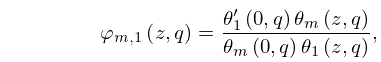
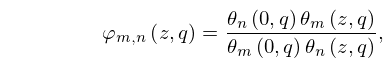
… ► … ►For $m=1,2,3,4$, $n=1,2,3,4$, and $m\ne n$, define twelve combined theta functions ${\phi }_{m,n}(z,q)$ by ►

20.11.6 $${\phi }_{m,1}(z,q)=\frac{{\theta }_1^{\prime }(0,q){\theta }_m(z,q)}{{\theta }_m(0,q){\theta }_1(z,q)},$$ $m=2,3,4$,

ⓘ

Symbols:

${\theta }_j(z,q)$: theta function, ${\phi }_{n,m}(z,q)$: combined theta function, $m$: integer, $z$: complex and $q$: nome

Permalink:

http://dlmf.nist.gov/20.11.E6

Encodings:

pMML, png, TeX

See also:

Annotations for §20.11(v), §20.11 and Ch.20

►

20.11.7 $${\phi }_{1,n}(z,q)=\frac{{\theta }_n(0,q){\theta }_1(z,q)}{{\theta }_1^{\prime }(0,q){\theta }_n(z,q)},$$ $n=2,3,4$,

ⓘ

Symbols:

${\theta }_j(z,q)$: theta function, ${\phi }_{n,m}(z,q)$: combined theta function, $n$: integer, $z$: complex and $q$: nome

Permalink:

http://dlmf.nist.gov/20.11.E7

Encodings:

pMML, png, TeX

See also:

Annotations for §20.11(v), §20.11 and Ch.20

►

20.11.8 $${\phi }_{m,n}(z,q)=\frac{{\theta }_n(0,q){\theta }_m(z,q)}{{\theta }_m(0,q){\theta }_n(z,q)},$$ $m,n=2,3,4$.

ⓘ

Symbols:

${\theta }_j(z,q)$: theta function, ${\phi }_{n,m}(z,q)$: combined theta function, $m$: integer, $n$: integer, $z$: complex and $q$: nome

Permalink:

http://dlmf.nist.gov/20.11.E8

Encodings:

pMML, png, TeX

See also:

Annotations for §20.11(v), §20.11 and Ch.20

…

2: 20.2 Definitions and Periodic Properties

… ►

§20.2(i) Fourier Series

►

20.2.1 $${\theta }_1\left(z\right|\tau )={\theta }_1(z,q)=2\sum _{n=0}^{\mathrm{\infty }}{(-1)}^n{q}^{{(n+\frac{1}{2})}^2}\sin \left((2n+1)z\right),$$

ⓘ

Symbols:

${\theta }_j(z,q)$: theta function, ${\theta }_j\left(z\right|\tau )$: theta function, $\sin z$: sine function, $n$: integer, $z$: complex, $\tau$: lattice parameter and $q$: nome

A&S Ref:

16.27.1

Referenced by:

§20.14, §20.2(i)

Permalink:

http://dlmf.nist.gov/20.2.E1

Encodings:

pMML, png, TeX

See also:

Annotations for §20.2(i), §20.2 and Ch.20

►

20.2.2 $${\theta }_2\left(z\right|\tau )={\theta }_2(z,q)=2\sum _{n=0}^{\mathrm{\infty }}{q}^{{(n+\frac{1}{2})}^2}\cos \left((2n+1)z\right),$$

ⓘ

Symbols:

${\theta }_j(z,q)$: theta function, ${\theta }_j\left(z\right|\tau )$: theta function, $\cos z$: cosine function, $n$: integer, $z$: complex, $\tau$: lattice parameter and $q$: nome

A&S Ref:

16.27.2

Permalink:

http://dlmf.nist.gov/20.2.E2

Encodings:

pMML, png, TeX

See also:

Annotations for §20.2(i), §20.2 and Ch.20

►

20.2.3 $${\theta }_3\left(z\right|\tau )={\theta }_3(z,q)=1+2\sum _{n=1}^{\mathrm{\infty }}{q}^{n^2}\cos \left(2nz\right),$$

ⓘ

Symbols:

${\theta }_j(z,q)$: theta function, ${\theta }_j\left(z\right|\tau )$: theta function, $\cos z$: cosine function, $n$: integer, $z$: complex, $\tau$: lattice parameter and $q$: nome

A&S Ref:

16.27.3

Referenced by:

§20.10(i), §20.13, §20.14, §27.13(iv)

Permalink:

http://dlmf.nist.gov/20.2.E3

Encodings:

pMML, png, TeX

See also:

Annotations for §20.2(i), §20.2 and Ch.20

►

20.2.4 $${\theta }_4\left(z\right|\tau )={\theta }_4(z,q)=1+2\sum _{n=1}^{\mathrm{\infty }}{(-1)}^n{q}^{n^2}\cos \left(2nz\right).$$

ⓘ

Symbols:

${\theta }_j(z,q)$: theta function, ${\theta }_j\left(z\right|\tau )$: theta function, $\cos z$: cosine function, $n$: integer, $z$: complex, $\tau$: lattice parameter and $q$: nome

A&S Ref:

16.27.4

Referenced by:

§20.13, §20.2(i)

Permalink:

http://dlmf.nist.gov/20.2.E4

Encodings:

pMML, png, TeX

See also:

Annotations for §20.2(i), §20.2 and Ch.20

…

3: 22.2 Definitions

… ►

22.2.4 $$\mathrm{sn}(z,k)=\frac{{\theta }_3(0,q)}{{\theta }_2(0,q)}\frac{{\theta }_1(\zeta ,q)}{{\theta }_4(\zeta ,q)}=\frac{1}{\mathrm{ns}(z,k)},$$

ⓘ

Defines:

$\mathrm{ns}(z,k)$: Jacobian elliptic function and $\mathrm{sn}(z,k)$: Jacobian elliptic function

Symbols:

${\theta }_j(z,q)$: theta function, $q$: nome, $z$: complex, $k$: modulus and $\zeta$: change of variable

Referenced by:

§23.6(ii)

Permalink:

http://dlmf.nist.gov/22.2.E4

Encodings:

pMML, png, TeX

See also:

Annotations for §22.2 and Ch.22

►

22.2.5 $$\mathrm{cn}(z,k)=\frac{{\theta }_4(0,q)}{{\theta }_2(0,q)}\frac{{\theta }_2(\zeta ,q)}{{\theta }_4(\zeta ,q)}=\frac{1}{\mathrm{nc}(z,k)},$$

ⓘ

Defines:

$\mathrm{cn}(z,k)$: Jacobian elliptic function and $\mathrm{nc}(z,k)$: Jacobian elliptic function

Symbols:

${\theta }_j(z,q)$: theta function, $q$: nome, $z$: complex, $k$: modulus and $\zeta$: change of variable

Permalink:

http://dlmf.nist.gov/22.2.E5

Encodings:

pMML, png, TeX

See also:

Annotations for §22.2 and Ch.22

►

22.2.6 $$\mathrm{dn}(z,k)=\frac{{\theta }_4(0,q)}{{\theta }_3(0,q)}\frac{{\theta }_3(\zeta ,q)}{{\theta }_4(\zeta ,q)}=\frac{1}{\mathrm{nd}(z,k)},$$

ⓘ

Defines:

$\mathrm{dn}(z,k)$: Jacobian elliptic function and $\mathrm{nd}(z,k)$: Jacobian elliptic function

Symbols:

${\theta }_j(z,q)$: theta function, $q$: nome, $z$: complex, $k$: modulus and $\zeta$: change of variable

Referenced by:

§22.20(ii)

Permalink:

http://dlmf.nist.gov/22.2.E6

Encodings:

pMML, png, TeX

See also:

Annotations for §22.2 and Ch.22

►

22.2.7 $$\mathrm{sd}(z,k)=\frac{{\theta }_3^2(0,q)}{{\theta }_2(0,q){\theta }_4(0,q)}\frac{{\theta }_1(\zeta ,q)}{{\theta }_3(\zeta ,q)}=\frac{1}{\mathrm{ds}(z,k)},$$

ⓘ

Defines:

$\mathrm{ds}(z,k)$: Jacobian elliptic function and $\mathrm{sd}(z,k)$: Jacobian elliptic function

Symbols:

${\theta }_j(z,q)$: theta function, $q$: nome, $z$: complex, $k$: modulus and $\zeta$: change of variable

Permalink:

http://dlmf.nist.gov/22.2.E7

Encodings:

pMML, png, TeX

See also:

Annotations for §22.2 and Ch.22

… ►

22.2.9 $$\mathrm{sc}(z,k)=\frac{{\theta }_3(0,q)}{{\theta }_4(0,q)}\frac{{\theta }_1(\zeta ,q)}{{\theta }_2(\zeta ,q)}=\frac{1}{\mathrm{cs}(z,k)}.$$

ⓘ

Defines:

$\mathrm{cs}(z,k)$: Jacobian elliptic function and $\mathrm{sc}(z,k)$: Jacobian elliptic function

Symbols:

${\theta }_j(z,q)$: theta function, $q$: nome, $z$: complex, $k$: modulus and $\zeta$: change of variable

Referenced by:

§23.6(ii)

Permalink:

http://dlmf.nist.gov/22.2.E9

Encodings:

pMML, png, TeX

See also:

Annotations for §22.2 and Ch.22

…

4: 23.15 Definitions

… ►

23.15.6 $$\lambda \left(\tau \right)=\frac{{\theta }_2^4(0,q)}{{\theta }_3^4(0,q)};$$

ⓘ

Defines:

$\lambda \left(\tau \right)$: elliptic modular function

Symbols:

${\theta }_j(z,q)$: theta function, $q$: nome and $\tau$: complex variable

Referenced by:

§20.9(ii), §23.17(iii)

Permalink:

http://dlmf.nist.gov/23.15.E6

Encodings:

pMML, png, TeX

See also:

Annotations for §23.15(ii), §23.15(ii), §23.15 and Ch.23

… ►

23.15.7 $$J\left(\tau \right)=\frac{{\left({\theta }_2^8(0,q)+{\theta }_3^8(0,q)+{\theta }_4^8(0,q)\right)}^3}{54{\left({\theta }_1^{\prime }(0,q)\right)}^8},$$

ⓘ

Defines:

$J\left(\tau \right)$: Klein’s complete invariant

Symbols:

${\theta }_j(z,q)$: theta function, $q$: nome and $\tau$: complex variable

Permalink:

http://dlmf.nist.gov/23.15.E7

Encodings:

pMML, png, TeX

See also:

Annotations for §23.15(ii), §23.15(ii), §23.15 and Ch.23

… ►

23.15.8 $${\theta }_1^{\prime }(0,q)={\partial {\theta }_1(z,q)/\partial z|}_{z=0}.$$

ⓘ

Symbols:

${\theta }_j(z,q)$: theta function, $\frac{\partial f}{\partial x}$: partial derivative of $f$ with respect to $x$ , $\partial x$: partial differential of $x$ , $q$: nome and $z$: complex

Permalink:

http://dlmf.nist.gov/23.15.E8

Encodings:

pMML, png, TeX

See also:

Annotations for §23.15(ii), §23.15(ii), §23.15 and Ch.23

… ►

23.15.9 $$\eta \left(\tau \right)={\left(\frac{1}{2}{\theta }_1^{\prime }(0,q)\right)}^{1/3}={\mathrm{e}}^{\mathrm{i}\pi \tau /12}{\theta }_3\left(\frac{1}{2}\pi (1+\tau )\right|3\tau ).$$

ⓘ

Symbols:

$\eta \left(\tau \right)$: Dedekind’s eta function (or Dedekind modular function), ${\theta }_j(z,q)$: theta function, ${\theta }_j\left(z\right|\tau )$: theta function, $\pi$: the ratio of the circumference of a circle to its diameter, $\mathrm{e}$: base of natural logarithm, $\mathrm{i}$: imaginary unit, $q$: nome and $\tau$: complex variable

Referenced by:

§23.15(ii), §23.15(ii), §23.17(iii)

Permalink:

http://dlmf.nist.gov/23.15.E9

Encodings:

pMML, png, TeX

See also:

Annotations for §23.15(ii), §23.15(ii), §23.15 and Ch.23

…

5: 20.15 Tables

… ►

20.15.1 $$\sin \alpha ={\theta }_2^2(0,q)/{\theta }_3^2(0,q)=k.$$

ⓘ

Defines:

$\alpha$: modular angle (locally)

Symbols:

${\theta }_j(z,q)$: theta function, $\sin z$: sine function and $q$: nome

Referenced by:

§20.15, §20.15

Permalink:

http://dlmf.nist.gov/20.15.E1

Encodings:

pMML, png, TeX

See also:

Annotations for §20.15 and Ch.20

… ►Tables of Neville’s theta functions ${\theta }_s(x,q)$, ${\theta }_c(x,q)$, ${\theta }_d(x,q)$, ${\theta }_n(x,q)$ (see §20.1) and their logarithmic $x$-derivatives are given in Abramowitz and Stegun (1964, pp. 582–585) to 9D for $\epsilon ,\alpha =0(5^{\circ }){90}^{\circ }$, where (in radian measure) $\epsilon =x/{\theta }_3^2(0,q)=\pi x/(2K\left(k\right))$, and $\alpha$ is defined by (20.15.1). …

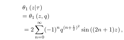
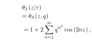
6: 20.1 Special Notation

… ►The main functions treated in this chapter are the theta functions ${\theta }_j\left(z\right|\tau )={\theta }_j(z,q)$ where $j=1,2,3,4$ and $q={\mathrm{e}}^{\mathrm{i}\pi \tau }$. … ►Primes on the $\theta$ symbols indicate derivatives with respect to the argument of the $\theta$ function. … ►Jacobi’s original notation: $\mathrm{\Theta }(z|\tau )$, ${\mathrm{\Theta }}_1(z|\tau )$, $\mathrm{H}(z|\tau )$, ${\mathrm{H}}_1(z|\tau )$, respectively, for ${\theta }_4\left(u\right|\tau )$, ${\theta }_3\left(u\right|\tau )$, ${\theta }_1\left(u\right|\tau )$, ${\theta }_2\left(u\right|\tau )$, where $u=z/{\theta }_3^2\left(0\right|\tau )$. 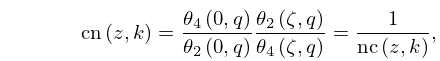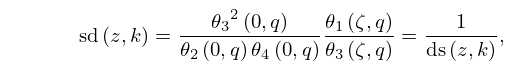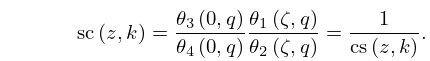… ►Neville’s notation: ${\theta }_s(z|\tau )$, ${\theta }_c(z|\tau )$, ${\theta }_d(z|\tau )$, ${\theta }_n(z|\tau )$, respectively, for ${\theta }_3^2\left(0\right|\tau ){\theta }_1\left(u\right|\tau )/{\theta }_1^{\prime }\left(0\right|\tau )$, ${\theta }_2\left(u\right|\tau )/{\theta }_2\left(0\right|\tau )$, ${\theta }_3\left(u\right|\tau )/{\theta }_3\left(0\right|\tau )$, ${\theta }_4\left(u\right|\tau )/{\theta }_4\left(0\right|\tau )$, where again $u=z/{\theta }_3^2\left(0\right|\tau )$. … ►McKean and Moll’s notation: ${\vartheta }_j(z|\tau )={\theta }_j\left(\pi z\right|\tau )$, $j=1,2,3,4$. …

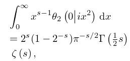
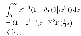
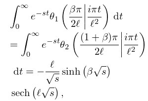
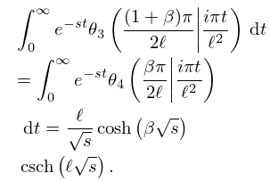
7: 20.10 Integrals

… ►

20.10.1 $${\int }_0^{\mathrm{\infty }}{x}^{s-1}{\theta }_2\left(0\right|\mathrm{i}{x}^2)dx=2^s(1-2^{-s}){\pi }^{-s/2}\mathrm{\Gamma }\left(\frac{1}{2}s\right)\zeta \left(s\right),$$ $\mathrm{\Re }s>1$,

ⓘ

Symbols:

$\mathrm{\Gamma }\left(z\right)$: gamma function, ${\theta }_j\left(z\right|\tau )$: theta function, $\zeta \left(s\right)$: Riemann zeta function, $\pi$: the ratio of the circumference of a circle to its diameter, $dx$: differential of $x$ , $\mathrm{i}$: imaginary unit, $\int$: integral and $\mathrm{\Re }$: real part

Keywords:

Mellin transform

Referenced by:

§20.10(i), Erratum (V1.1.5) for §20.10(i)

Permalink:

http://dlmf.nist.gov/20.10.E1

Encodings:

pMML, png, TeX

Modification (effective with 1.1.5):

Originally the constraint was $\mathrm{\Re }s>2$. This can be relaxed to $\mathrm{\Re }s>1$ because ${\theta }_2\left(0\right|\mathrm{i}{x}^2)=x^{-1}{\theta }_4\left(0\right|\mathrm{i}{x}^{-2})\sim x^{-1}$ as $x\to 0+$, which follows from (20.7.31) and (20.4.5).

See also:

Annotations for §20.10(i), §20.10 and Ch.20

►

20.10.2 $${\int }_0^{\mathrm{\infty }}{x}^{s-1}({\theta }_3\left(0\right|\mathrm{i}{x}^2)-1)dx={\pi }^{-s/2}\mathrm{\Gamma }\left(\frac{1}{2}s\right)\zeta \left(s\right),$$ $\mathrm{\Re }s>1$,

ⓘ

Symbols:

$\mathrm{\Gamma }\left(z\right)$: gamma function, ${\theta }_j\left(z\right|\tau )$: theta function, $\zeta \left(s\right)$: Riemann zeta function, $\pi$: the ratio of the circumference of a circle to its diameter, $dx$: differential of $x$ , $\mathrm{i}$: imaginary unit, $\int$: integral and $\mathrm{\Re }$: real part

Keywords:

Mellin transform

Referenced by:

§20.10(i), Erratum (V1.1.5) for §20.10(i)

Permalink:

http://dlmf.nist.gov/20.10.E2

Encodings:

pMML, png, TeX

Modification (effective with 1.1.5):

Originally the constraint was $\mathrm{\Re }s>2$. This can be relaxed to $\mathrm{\Re }s>1$ because ${\theta }_3\left(0\right|\mathrm{i}{x}^2)=x^{-1}{\theta }_3\left(0\right|\mathrm{i}{x}^{-2})\sim x^{-1}$ as $x\to 0+$, which follows from (20.7.32) and (20.4.4).

See also:

Annotations for §20.10(i), §20.10 and Ch.20

►

20.10.3 $${\int }_0^{\mathrm{\infty }}{x}^{s-1}(1-{\theta }_4\left(0\right|\mathrm{i}{x}^2))dx=(1-2^{1-s}){\pi }^{-s/2}\mathrm{\Gamma }\left(\frac{1}{2}s\right)\zeta \left(s\right),$$ $\mathrm{\Re }s>0$.

ⓘ

Symbols:

$\mathrm{\Gamma }\left(z\right)$: gamma function, ${\theta }_j\left(z\right|\tau )$: theta function, $\zeta \left(s\right)$: Riemann zeta function, $\pi$: the ratio of the circumference of a circle to its diameter, $dx$: differential of $x$ , $\mathrm{i}$: imaginary unit, $\int$: integral and $\mathrm{\Re }$: real part

Keywords:

Mellin transform

Referenced by:

§20.10(i), Erratum (V1.1.5) for §20.10(i)

Permalink:

http://dlmf.nist.gov/20.10.E3

Encodings:

pMML, png, TeX

Modification (effective with 1.1.5):

Originally the constraint was $\mathrm{\Re }s>2$. This can be relaxed to $\mathrm{\Re }s>0$ because $1-{\theta }_4\left(0\right|\mathrm{i}{x}^2)=1-x^{-1}{\theta }_2\left(0\right|\mathrm{i}{x}^{-2})\sim 1$ as $x\to 0+$, which follows from (20.7.33) and (20.4.3).

See also:

Annotations for §20.10(i), §20.10 and Ch.20

… ►

20.10.4 $${\int }_0^{\mathrm{\infty }}{\mathrm{e}}^{-st}{\theta }_1\left(\frac{\beta \pi }{2\mathrm{\ell }}\right|\frac{\mathrm{i}\pi t}{{\mathrm{\ell }}^2})dt={\int }_0^{\mathrm{\infty }}{\mathrm{e}}^{-st}{\theta }_2\left(\frac{(1+\beta )\pi }{2\mathrm{\ell }}\right|\frac{\mathrm{i}\pi t}{{\mathrm{\ell }}^2})dt=-\frac{\mathrm{\ell }}{\sqrt{s}}\sinh \left(\beta \sqrt{s}\right)\mathrm{sech}\left(\mathrm{\ell }\sqrt{s}\right),$$

ⓘ

Symbols:

${\theta }_j\left(z\right|\tau )$: theta function, $\pi$: the ratio of the circumference of a circle to its diameter, $dx$: differential of $x$ , $\mathrm{e}$: base of natural logarithm, $\mathrm{sech}z$: hyperbolic secant function, $\sinh z$: hyperbolic sine function, $\mathrm{i}$: imaginary unit, $\int$: integral, $s$: parameter, $\beta$: parameter and $\mathrm{\ell }$: parameter

Permalink:

http://dlmf.nist.gov/20.10.E4

Encodings:

pMML, png, TeX

See also:

Annotations for §20.10(ii), §20.10 and Ch.20

►

20.10.5 $${\int }_0^{\mathrm{\infty }}{\mathrm{e}}^{-st}{\theta }_3\left(\frac{(1+\beta )\pi }{2\mathrm{\ell }}\right|\frac{\mathrm{i}\pi t}{{\mathrm{\ell }}^2})dt={\int }_0^{\mathrm{\infty }}{\mathrm{e}}^{-st}{\theta }_4\left(\frac{\beta \pi }{2\mathrm{\ell }}\right|\frac{\mathrm{i}\pi t}{{\mathrm{\ell }}^2})dt=\frac{\mathrm{\ell }}{\sqrt{s}}\cosh \left(\beta \sqrt{s}\right)\mathrm{csch}\left(\mathrm{\ell }\sqrt{s}\right).$$

ⓘ

Symbols:

${\theta }_j\left(z\right|\tau )$: theta function, $\pi$: the ratio of the circumference of a circle to its diameter, $dx$: differential of $x$ , $\mathrm{e}$: base of natural logarithm, $\mathrm{csch}z$: hyperbolic cosecant function, $\cosh z$: hyperbolic cosine function, $\mathrm{i}$: imaginary unit, $\int$: integral, $s$: parameter, $\beta$: parameter and $\mathrm{\ell }$: parameter

Permalink:

http://dlmf.nist.gov/20.10.E5

Encodings:

pMML, png, TeX

See also:

Annotations for §20.10(ii), §20.10 and Ch.20

…

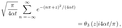
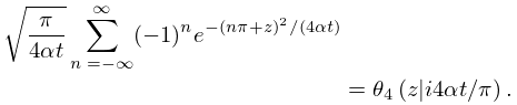
8: 20.13 Physical Applications

… ►The functions ${\theta }_j\left(z\right|\tau )$, $j=1,2,3,4$, provide periodic solutions of the partial differential equation … ►

20.13.4 $$\sqrt{\frac{\pi }{4\alpha t}}\sum _{n=-\mathrm{\infty }}^{\mathrm{\infty }}{\mathrm{e}}^{-{(n\pi +z)}^2/(4\alpha t)}={\theta }_3\left(z\right|\mathrm{i}4\alpha t/\pi ),$$

ⓘ

Symbols:

${\theta }_j\left(z\right|\tau )$: theta function, $\pi$: the ratio of the circumference of a circle to its diameter, $\mathrm{e}$: base of natural logarithm, $\mathrm{i}$: imaginary unit, $n$: integer, $t$: time, $\alpha$: real parameter and $z$: real variable

Permalink:

http://dlmf.nist.gov/20.13.E4

Encodings:

pMML, png, TeX

See also:

Annotations for §20.13 and Ch.20

… ►

20.13.5 $$\sqrt{\frac{\pi }{4\alpha t}}\sum _{n=-\mathrm{\infty }}^{\mathrm{\infty }}{(-1)}^n{\mathrm{e}}^{-{(n\pi +z)}^2/(4\alpha t)}={\theta }_4\left(z\right|\mathrm{i}4\alpha t/\pi ).$$

ⓘ

Symbols:

${\theta }_j\left(z\right|\tau )$: theta function, $\pi$: the ratio of the circumference of a circle to its diameter, $\mathrm{e}$: base of natural logarithm, $\mathrm{i}$: imaginary unit, $n$: integer, $t$: time, $\alpha$: real parameter and $z$: real variable

Permalink:

http://dlmf.nist.gov/20.13.E5

Encodings:

pMML, png, TeX

See also:

Annotations for §20.13 and Ch.20

… ►In the singular limit $\mathrm{\Im }\tau \to 0+$, the functions ${\theta }_j\left(z\right|\tau )$, $j=1,2,3,4$, become integral kernels of Feynman path integrals (distribution-valued Green’s functions); see Schulman (1981, pp. 194–195). …

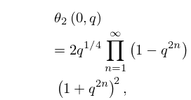
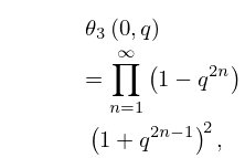
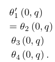
9: 20.4 Values at $z$ = 0

… ►

20.4.3 $${\theta }_2(0,q)=2q^{1/4}\prod _{n=1}^{\mathrm{\infty }}\left(1-q^{2n}\right){\left(1+q^{2n}\right)}^2,$$

ⓘ

Symbols:

${\theta }_j(z,q)$: theta function, $n$: integer and $q$: nome

Referenced by:

(20.10.3)

Permalink:

http://dlmf.nist.gov/20.4.E3

Encodings:

pMML, png, TeX

See also:

Annotations for §20.4(i), §20.4 and Ch.20

►

20.4.4 $${\theta }_3(0,q)=\prod _{n=1}^{\mathrm{\infty }}\left(1-q^{2n}\right){\left(1+q^{2n-1}\right)}^2,$$

ⓘ

Symbols:

${\theta }_j(z,q)$: theta function, $n$: integer and $q$: nome

Referenced by:

(20.10.2)

Permalink:

http://dlmf.nist.gov/20.4.E4

Encodings:

pMML, png, TeX

See also:

Annotations for §20.4(i), §20.4 and Ch.20

►

20.4.5 $${\theta }_4(0,q)=\prod _{n=1}^{\mathrm{\infty }}\left(1-q^{2n}\right){\left(1-q^{2n-1}\right)}^2.$$

ⓘ

Symbols:

${\theta }_j(z,q)$: theta function, $n$: integer and $q$: nome

Referenced by:

(20.10.1)

Permalink:

http://dlmf.nist.gov/20.4.E5

Encodings:

pMML, png, TeX

See also:

Annotations for §20.4(i), §20.4 and Ch.20

►

Jacobi’s Identity

►

20.4.6 $${\theta }_1^{\prime }(0,q)={\theta }_2(0,q){\theta }_3(0,q){\theta }_4(0,q).$$

ⓘ

Symbols:

${\theta }_j(z,q)$: theta function and $q$: nome

A&S Ref:

16.28.6

Referenced by:

§20.9(i)

Permalink:

http://dlmf.nist.gov/20.4.E6

Encodings:

pMML, png, TeX

See also:

Annotations for §20.4(i), §20.4(i), §20.4 and Ch.20

…

10: 20.8 Watson’s Expansions

… ►

20.8.1 $$\frac{{\theta }_2(0,q){\theta }_3(z,q){\theta }_4(z,q)}{{\theta }_2(z,q)}=2\sum _{n=-\mathrm{\infty }}^{\mathrm{\infty }}\frac{{(-1)}^n{q}^{n^2}{\mathrm{e}}^{\mathrm{i}2nz}}{q^{-n}{\mathrm{e}}^{-\mathrm{i}z}+q^n{\mathrm{e}}^{\mathrm{i}z}}.$$

ⓘ

Symbols:

${\theta }_j(z,q)$: theta function, $\mathrm{e}$: base of natural logarithm, $\mathrm{i}$: imaginary unit, $n$: integer, $z$: complex and $q$: nome

Permalink:

http://dlmf.nist.gov/20.8.E1

Encodings:

pMML, png, TeX

See also:

Annotations for §20.8 and Ch.20

…