Glaisher%20constant

SearchAdvancedHelp

(0.003 seconds)

1—10 of 501 matching pages

1: 5.17 Barnes’ $G$-Function (Double Gamma Function)

… ►

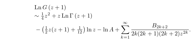
5.17.5 $$\mathrm{Ln}G\left(z+1\right)\sim \frac{1}{4}{z}^2+z\mathrm{Ln}\mathrm{\Gamma }\left(z+1\right)-\left(\frac{1}{2}z(z+1)+\frac{1}{12}\right)\ln z-\ln A+\sum _{k=1}^{\mathrm{\infty }}\frac{B_{2k+2}}{2k(2k+1)(2k+2)z^{2k}}.$$

ⓘ

Symbols:

$G\left(z\right)$: Barnes’ $G$-function (or double gamma function), $B_n$: Bernoulli numbers, $\mathrm{\Gamma }\left(z\right)$: gamma function, $\sim$: Poincaré asymptotic expansion, $\mathrm{Ln}z$: general logarithm function, $\ln z$: principal branch of logarithm function, $k$: nonnegative integer, $z$: complex variable and $A$: Glaisher’s constant

Referenced by:

§5.17, §5.17, Erratum (V1.0.7) for Equation (5.17.5), Erratum (V1.1.11) for Equation (5.17.5)

Permalink:

http://dlmf.nist.gov/5.17.E5

Encodings:

pMML, png, TeX

Errata (effective with 1.1.11):

For consistency we have replaced $\mathrm{Ln}z$ by $\ln z$.

Errata (effective with 1.0.7):

Originally the term $z\mathrm{Ln}\mathrm{\Gamma }\left(z+1\right)$ was incorrectly stated as $z\mathrm{\Gamma }\left(z+1\right)$. (This error was reported subsequently by Nick Jones on December 11, 2013.)

Reported 2013-08-01 by Gergő Nemes

See also:

Annotations for §5.17 and Ch.5

… ►Here $B_{2k+2}$ is the Bernoulli number (§24.2(i)), and $A$ is Glaisher’s constant, given by ►

5.17.6 $$A={\mathrm{e}}^C=\mathrm{1.28242\hspace{0.33em}71291\hspace{0.33em}00622\hspace{0.33em}63687}\mathrm{\dots },$$

ⓘ

Symbols:

$\mathrm{e}$: base of natural logarithm, $A$: Glaisher’s constant and $C$: log of Glaisher’s Constant

Notes:

For more digits see OEIS Sequence A074962; see also Sloane (2003).

Permalink:

http://dlmf.nist.gov/5.17.E6

Encodings:

pMML, png, TeX

See also:

Annotations for §5.17 and Ch.5

… ►

5.17.7 $$C=\underset{n\to \mathrm{\infty }}{lim}\left(\sum _{k=1}^{n}k\ln k-\left(\frac{1}{2}{n}^2+\frac{1}{2}n+\frac{1}{12}\right)\ln n+\frac{1}{4}{n}^2\right)=\frac{\gamma +\ln \left(2\pi \right)}{12}-\frac{{\zeta }^{\prime }\left(2\right)}{2{\pi }^2}=\frac{1}{12}-{\zeta }^{\prime }\left(-1\right),$$

ⓘ

Symbols:

$\gamma$: Euler’s constant, $\zeta \left(s\right)$: Riemann zeta function, $\pi$: the ratio of the circumference of a circle to its diameter, $\ln z$: principal branch of logarithm function, $n$: nonnegative integer, $k$: nonnegative integer and $C$: log of Glaisher’s Constant

Referenced by:

§5.17

Permalink:

http://dlmf.nist.gov/5.17.E7

Encodings:

pMML, png, TeX

See also:

Annotations for §5.17 and Ch.5

… ►For Glaisher’s constant see also Greene and Knuth (1982, p. 100) and §2.10(i).

2: 22.1 Special Notation

… ►The notation $\mathrm{sn}(z,k)$, $\mathrm{cn}(z,k)$, $\mathrm{dn}(z,k)$ is due to Gudermann (1838), following Jacobi (1827); that for the subsidiary functions is due to Glaisher (1882). Other notations for $\mathrm{sn}(z,k)$ are $\mathrm{sn}(z|m)$ and $\mathrm{sn}(z,m)$ with $m=k^2$; see Abramowitz and Stegun (1964) and Walker (1996). …

3: 27.21 Tables

… ►Glaisher (1940) contains four tables: Table I tabulates, for all $n\le {10}^4$: (a) the canonical factorization of $n$ into powers of primes; (b) the Euler totient $\varphi \left(n\right)$; (c) the divisor function $d\left(n\right)$; (d) the sum $\sigma (n)$ of these divisors. …7 of Abramowitz and Stegun (1964) also lists the factorizations in Glaisher’s Table I(a); Table 24. …

4: 2.10 Sums and Sequences

… ►Formula (2.10.2) is useful for evaluating the constant term in expansions obtained from (2.10.1). …where $\gamma$ is Euler’s constant (§5.2(ii)) and ${\zeta }^{\prime }$ is the derivative of the Riemann zeta function (§25.2(i)). ${\mathrm{e}}^C$ is sometimes called Glaisher’s constant. … ►where $\alpha$ ($\ne -1$) is a real constant, and … ►for any real constant $\alpha$ and the set of all positive integers $j$, we derive …

5: 8.26 Tables

… ►

Khamis (1965) tabulates $P(a,x)$ for $a=0.05(.05)10(.1)20(.25)70$, $0.0001\le x\le 250$ to 10D.

… ►

Zhang and Jin (1996, Table 3.8) tabulates $\gamma (a,x)$ for $a=0.5,1,3,5,10,25,50,100$, $x=0(.1)1(1)3,5(5)30,50,100$ to 8D or 8S.

… ►

Abramowitz and Stegun (1964, pp. 245–248) tabulates $E_n\left(x\right)$ for $n=2,3,4,10,20$, $x=0(.01)2$ to 7D; also $(x+n){\mathrm{e}}^x{E}_n\left(x\right)$ for $n=2,3,4,10,20$, $x^{-1}=0(.01)0.1(.05)0.5$ to 6S.

… ►

Pagurova (1961) tabulates $E_n\left(x\right)$ for $n=0(1)20$, $x=0(.01)2(.1)10$ to 4-9S; ${\mathrm{e}}^x{E}_n\left(x\right)$ for $n=2(1)10$, $x=10(.1)20$ to 7D; ${\mathrm{e}}^x{E}_p\left(x\right)$ for $p=0(.1)1$, $x=0.01(.01)7(.05)12(.1)20$ to 7S or 7D.

… ►

Zhang and Jin (1996, Table 19.1) tabulates $E_n\left(x\right)$ for $n=1,2,3,5,10,15,20$, $x=0(.1)1,1.5,2,3,5,10,20,30,50,100$ to 7D or 8S.

6: 20 Theta Functions

Chapter 20 Theta Functions

…

7: Bibliography G

… ►

Algorithm 726: ORTHPOL — a package of routines for generating orthogonal polynomials and Gauss-type quadrature rules. ACM Trans. Math. Software 20 (1), pp. 21–62.

ⓘ

Notes:

For remark see same journal 24(1998), p. 355.

External Links:

Document, ISSN 0098-3500, GAMS (module 726; package TOMS), ZentralBlatt

Referenced by:

2nd item, §3.5(v), §3.5(v).

Encodings:

BibTeX

… ►

Algorithm 939: computation of the Marcum Q-function. ACM Trans. Math. Softw. 40 (3), pp. 20:1–20:21.

ⓘ

Notes:

Includes Fortran program claiming 12S accuracy

External Links:

ISSN 0098-3500, Link, Document, MathReview Entry, ZentralBlatt

Referenced by:

3rd item, §10.77(ix).

Encodings:

BibTeX

… ►

Number-Divisor Tables. British Association Mathematical Tables, Vol. VIII, Cambridge University Press, Cambridge, England.

ⓘ

External Links:

MathReview (D. H. Lehmer), ZentralBlatt

Referenced by:

§27.21.

Encodings:

BibTeX

… ►

Mutual integrability, quadratic algebras, and dynamical symmetry. Ann. Phys. 217 (1), pp. 1–20.

ⓘ

External Links:

ISSN 0003-4916, Link, MathReview (A. O. Barut), ZentralBlatt

Referenced by:

§18.38(iii).

Encodings:

BibTeX

…

8: 22.4 Periods, Poles, and Zeros

… ►

§22.4(ii) Graphical Interpretation via Glaisher’s Notation

…

9: 20.7 Identities

… ►Also, in further development along the lines of the notations of Neville (§20.1) and of Glaisher (§22.2), the identities (20.7.6)–(20.7.9) have been recast in a more symmetric manner with respect to suffices $2,3,4$. … ►See Lawden (1989, pp. 19–20). … ►

20.7.34 $$\frac{{\theta }_1(z,q^2){\theta }_3(z,q^2)}{{\theta }_1(z,\mathrm{i}q)}=\frac{{\theta }_2(z,q^2){\theta }_4(z,q^2)}{{\theta }_2(z,\mathrm{i}q)}={\mathrm{i}}^{-1/4}\sqrt{\frac{{\theta }_2(0,q^2){\theta }_4(0,q^2)}{2}}.$$

ⓘ

Symbols:

${\theta }_j(z,q)$: theta function, $\mathrm{i}$: imaginary unit, $z$: complex and $q$: nome

Referenced by:

§20.7(iv), Erratum (V1.0.5) for Chapters 8, 20, 36

Permalink:

http://dlmf.nist.gov/20.7.E34

Encodings:

pMML, png, TeX

Addition (effective with 1.0.5):

This equation has been added. See Walker (2012).

See also:

Annotations for §20.7(ix), §20.7 and Ch.20

…

10: 5.22 Tables

… ►Abramowitz and Stegun (1964, Chapter 6) tabulates $\mathrm{\Gamma }\left(x\right)$, $\ln \mathrm{\Gamma }\left(x\right)$, $\psi \left(x\right)$, and ${\psi }^{\prime }\left(x\right)$ for $x=1(.005)2$ to 10D; ${\psi }^{\prime \prime }\left(x\right)$ and ${\psi }^{(3)}\left(x\right)$ for $x=1(.01)2$ to 10D; $\mathrm{\Gamma }\left(n\right)$, $1/\mathrm{\Gamma }\left(n\right)$, $\mathrm{\Gamma }\left(n+\frac{1}{2}\right)$, $\psi \left(n\right)$, ${\log }_{10}\mathrm{\Gamma }\left(n\right)$, ${\log }_{10}\mathrm{\Gamma }\left(n+\frac{1}{3}\right)$, ${\log }_{10}\mathrm{\Gamma }\left(n+\frac{1}{2}\right)$, and ${\log }_{10}\mathrm{\Gamma }\left(n+\frac{2}{3}\right)$ for $n=1(1)101$ to 8–11S; $\mathrm{\Gamma }\left(n+1\right)$ for $n=100(100)1000$ to 20S. Zhang and Jin (1996, pp. 67–69 and 72) tabulates $\mathrm{\Gamma }\left(x\right)$, $1/\mathrm{\Gamma }\left(x\right)$, $\mathrm{\Gamma }\left(-x\right)$, $\ln \mathrm{\Gamma }\left(x\right)$, $\psi \left(x\right)$, $\psi \left(-x\right)$, ${\psi }^{\prime }\left(x\right)$, and ${\psi }^{\prime }\left(-x\right)$ for $x=0(.1)5$ to 8D or 8S; $\mathrm{\Gamma }\left(n+1\right)$ for $n=0(1)100(10)250(50)500(100)3000$ to 51S. … ►Abramov (1960) tabulates $\ln \mathrm{\Gamma }\left(x+\mathrm{i}y\right)$ for $x=1$ ($.01$) $2$, $y=0$ ($.01$) $4$ to 6D. Abramowitz and Stegun (1964, Chapter 6) tabulates $\ln \mathrm{\Gamma }\left(x+\mathrm{i}y\right)$ for $x=1$ ($.1$) $2$, $y=0$ ($.1$) $10$ to 12D. …Zhang and Jin (1996, pp. 70, 71, and 73) tabulates the real and imaginary parts of $\mathrm{\Gamma }\left(x+\mathrm{i}y\right)$, $\ln \mathrm{\Gamma }\left(x+\mathrm{i}y\right)$, and $\psi \left(x+\mathrm{i}y\right)$ for $x=0.5,1,5,10$, $y=0(.5)10$ to 8S.