Gibbs phenomenon

SearchAdvancedHelp

(0.002 seconds)

1—10 of 16 matching pages

1: 6.16 Mathematical Applications

… ►

§6.16(i) The Gibbs Phenomenon

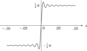
… ►This nonuniformity of convergence is an illustration of the Gibbs phenomenon. … ►

►►

Figure 6.16.1: Graph of $S_n(x)$, $n=250$, $-0.1\le x\le 0.1$, illustrating the Gibbs phenomenon. Magnify

…

2: Sidebar 9.SB1: Supernumerary Rainbows

… ►Airy invented his function in 1838 precisely to describe this phenomenon more accurately than Young had done in 1800 when pointing out that supernumerary rainbows require the wave theory of light and are impossible to explain with Newton’s picture of light as a stream of independent corpuscles. …

3: 7.20 Mathematical Applications

… ►For applications of the complementary error function in uniform asymptotic approximations of integrals—saddle point coalescing with a pole or saddle point coalescing with an endpoint—see Wong (1989, Chapter 7), Olver (1997b, Chapter 9), and van der Waerden (1951). ►The complementary error function also plays a ubiquitous role in constructing exponentially-improved asymptotic expansions and providing a smooth interpretation of the Stokes phenomenon; see §§2.11(iii) and 2.11(iv). …

4: 8.22 Mathematical Applications

… ►

8.22.1 $$F_p\left(z\right)=\frac{\mathrm{\Gamma }\left(p\right)}{2\pi }{z}^{1-p}{E}_p\left(z\right)=\frac{\mathrm{\Gamma }\left(p\right)}{2\pi }\mathrm{\Gamma }(1-p,z),$$

ⓘ

Symbols:

$\mathrm{\Gamma }\left(z\right)$: gamma function, $\pi$: the ratio of the circumference of a circle to its diameter, $E_p\left(z\right)$: generalized exponential integral, $\mathrm{\Gamma }(a,z)$: incomplete gamma function, $F_p\left(z\right)$: terminant function, $z$: complex variable and $p$: parameter

Permalink:

http://dlmf.nist.gov/8.22.E1

Encodings:

pMML, png, TeX

See also:

Annotations for §8.22(i), §8.22 and Ch.8

►plays a fundamental role in re-expansions of remainder terms in asymptotic expansions, including exponentially-improved expansions and a smooth interpretation of the Stokes phenomenon. …

5: Bibliography P

… ►

Stokes phenomenon demystified. Bull. Inst. Math. Appl. 31 (1-2), pp. 21–28.

ⓘ

External Links:

ISSN 0905-5628, MathReview Entry, ZentralBlatt

Referenced by:

§2.11(iv).

Encodings:

BibTeX

… ►

Smoothing of the Stokes phenomenon for high-order differential equations. Proc. Roy. Soc. London Ser. A 436, pp. 165–186.

ⓘ

External Links:

ISSN 0962-8444, FullText, MathReview (F. W. J. Olver), ZentralBlatt

Referenced by:

§2.11(v).

Encodings:

BibTeX

►

Smoothing of the Stokes phenomenon using Mellin-Barnes integrals. J. Comput. Appl. Math. 41 (1-2), pp. 117–133.

ⓘ

External Links:

ISSN 0377-0427, Document, MathReview (Anatoly Kilbas), ZentralBlatt

Referenced by:

§2.11(v).

Encodings:

BibTeX

… ►

The Stokes phenomenon associated with the Hurwitz zeta function $\zeta (s,a)$ . Proc. Roy. Soc. London Ser. A 461, pp. 297–304.

ⓘ

External Links:

ISSN 1364-5021, Document, MathReview (Marc Prevost), ZentralBlatt

Referenced by:

(25.11.43), §25.11(xii).

Encodings:

BibTeX

…

6: 9.10 Integrals

… ►

9.10.14 $${\int }_0^{\mathrm{\infty }}{\mathrm{e}}^{-pt}\mathrm{Ai}\left(t\right)dt={\mathrm{e}}^{-p^3/3}\left(\frac{1}{3}-\frac{p{}_1{}^{}F_1^{}(\frac{1}{3};\frac{4}{3};\frac{1}{3}{p}^3)}{3^{4/3}\mathrm{\Gamma }\left(\frac{4}{3}\right)}+\frac{p^2{}_1{}^{}F_1^{}(\frac{2}{3};\frac{5}{3};\frac{1}{3}{p}^3)}{3^{5/3}\mathrm{\Gamma }\left(\frac{5}{3}\right)}\right),$$ $p\in ℂ$.

ⓘ

Symbols:

$\mathrm{Ai}\left(z\right)$: Airy function, $\mathrm{\Gamma }\left(z\right)$: gamma function, ${}_1{}^{}F_1^{}(a;b;z)$: $=M(a,b,z)$ notation for the Kummer confluent hypergeometric function, $ℂ$: complex plane, $dx$: differential of $x$ , $\in$: element of, $\mathrm{e}$: base of natural logarithm, $\int$: integral and $p$: parameter

Keywords:

Laplace transform

Source:

Gibbs (1973, Problem 72–21)

Permalink:

http://dlmf.nist.gov/9.10.E14

Encodings:

pMML, png, TeX

See also:

Annotations for §9.10(v), §9.10 and Ch.9

►

9.10.15 $${\int }_0^{\mathrm{\infty }}{\mathrm{e}}^{-pt}\mathrm{Ai}\left(-t\right)dt=\frac{1}{3}{\mathrm{e}}^{p^3/3}\left(\frac{\mathrm{\Gamma }(\frac{1}{3},\frac{1}{3}{p}^3)}{\mathrm{\Gamma }\left(\frac{1}{3}\right)}+\frac{\mathrm{\Gamma }(\frac{2}{3},\frac{1}{3}{p}^3)}{\mathrm{\Gamma }\left(\frac{2}{3}\right)}\right),$$ $\mathrm{\Re }p>0$,

ⓘ

Symbols:

$\mathrm{Ai}\left(z\right)$: Airy function, $\mathrm{\Gamma }\left(z\right)$: gamma function, $dx$: differential of $x$ , $\mathrm{e}$: base of natural logarithm, $\mathrm{\Gamma }(a,z)$: incomplete gamma function, $\int$: integral, $\mathrm{\Re }$: real part and $p$: parameter

Keywords:

Laplace transform

Source:

Gibbs (1973, Problem 72–21)

Permalink:

http://dlmf.nist.gov/9.10.E15

Encodings:

pMML, png, TeX

See also:

Annotations for §9.10(v), §9.10 and Ch.9

►

9.10.16 $${\int }_0^{\mathrm{\infty }}{\mathrm{e}}^{-pt}\mathrm{Bi}\left(-t\right)dt=\frac{1}{\sqrt{3}}{\mathrm{e}}^{p^3/3}\left(\frac{\mathrm{\Gamma }(\frac{2}{3},\frac{1}{3}{p}^3)}{\mathrm{\Gamma }\left(\frac{2}{3}\right)}-\frac{\mathrm{\Gamma }(\frac{1}{3},\frac{1}{3}{p}^3)}{\mathrm{\Gamma }\left(\frac{1}{3}\right)}\right),$$ $\mathrm{\Re }p>0$.

ⓘ

Symbols:

$\mathrm{Bi}\left(z\right)$: Airy function, $\mathrm{\Gamma }\left(z\right)$: gamma function, $dx$: differential of $x$ , $\mathrm{e}$: base of natural logarithm, $\mathrm{\Gamma }(a,z)$: incomplete gamma function, $\int$: integral, $\mathrm{\Re }$: real part and $p$: parameter

Keywords:

Laplace transform

Source:

Gibbs (1973, Problem 72–21)

Permalink:

http://dlmf.nist.gov/9.10.E16

Encodings:

pMML, png, TeX

See also:

Annotations for §9.10(v), §9.10 and Ch.9

…

7: 2.11 Remainder Terms; Stokes Phenomenon

§2.11 Remainder Terms; Stokes Phenomenon

… ►

§2.11(iv) Stokes Phenomenon

… ►That the change in their forms is discontinuous, even though the function being approximated is analytic, is an example of the Stokes phenomenon. Where should the change-over take place? Can it be accomplished smoothly? …

8: 10.46 Generalized and Incomplete Bessel Functions; Mittag-Leffler Function

… ►For exponentially-improved asymptotic expansions in the same circumstances, together with smooth interpretations of the corresponding Stokes phenomenon (§§2.11(iii)–2.11(v)) see Wong and Zhao (1999b) when $\rho >0$, and Wong and Zhao (1999a) when . …

9: Bibliography I

… ►

Quasi-linear Stokes phenomenon for the second Painlevé transcendent. Nonlinearity 16 (1), pp. 363–386.

ⓘ

External Links:

ISSN 0951-7715, Document, MathReview (Youmin Lu), ZentralBlatt

Referenced by:

§32.12(ii).

Encodings:

BibTeX

…

10: 7.12 Asymptotic Expansions

… ►For these and other error bounds see Olver (1997b, pp. 109–112), with $\alpha =\frac{1}{2}$ and $z$ replaced by $z^2$; compare (7.11.2). ►For re-expansions of the remainder terms leading to larger sectors of validity, exponential improvement, and a smooth interpretation of the Stokes phenomenon, see §§2.11(ii)–2.11(iv) and use (7.11.3). …