Gauss%E2%80%93Legendre%20formula
(0.004 seconds)
1—10 of 462 matching pages
1: 14.1 Special Notation
§14.1 Special Notation
… ►The main functions treated in this chapter are the Legendre functions , , , ; Ferrers functions , (also known as the Legendre functions on the cut); associated Legendre functions , , ; conical functions , , , , (also known as Mehler functions). … ►Magnus et al. (1966) denotes , , , and by , , , and , respectively. Hobson (1931) denotes both and by ; similarly for and .2: 18.3 Definitions
§18.3 Definitions
… ►This table also includes the following special cases of Jacobi polynomials: ultraspherical, Chebyshev, and Legendre. … ►Formula (18.3.1) can be understood as a Gauss-Chebyshev quadrature, see (3.5.22), (3.5.23). … ►Legendre
►Legendre polynomials are special cases of Legendre functions, Ferrers functions, and associated Legendre functions (§14.7(i)). …3: 15.5 Derivatives and Contiguous Functions
…
►
§15.5(i) Differentiation Formulas
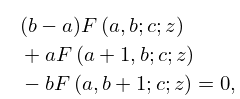
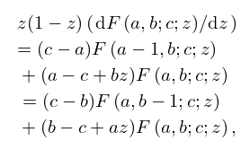
… ►The six functions , , are said to be contiguous to . … ►
15.5.12
…
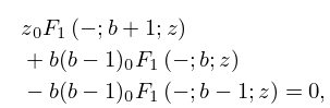
►By repeated applications of (15.5.11)–(15.5.18) any function , in which are integers, can be expressed as a linear combination of and any one of its contiguous functions, with coefficients that are rational functions of , and .
…
►
15.5.20
…
4: 16.12 Products
…
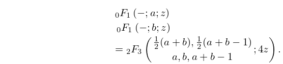
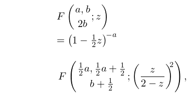
►
16.12.1
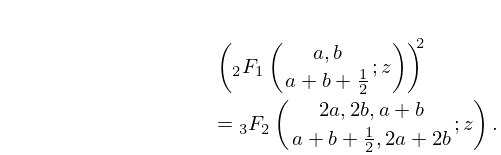
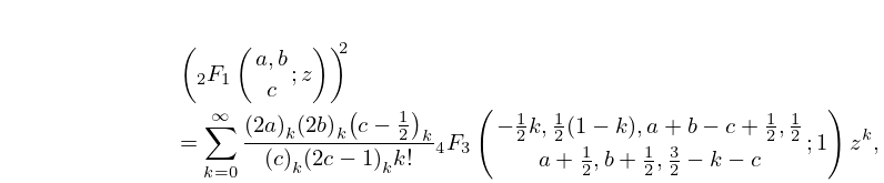
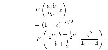
►The following formula is often referred to as Clausen’s formula
►
16.12.2
…
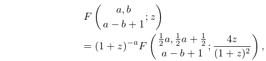
►
16.12.3
.
…
5: 15.4 Special Cases
6: 15.16 Products
7: 15.2 Definitions and Analytical Properties
…
►
§15.2(i) Gauss Series
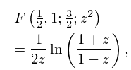
►The hypergeometric function is defined by the Gauss series … ►On the circle of convergence, , the Gauss series: … ►The same properties hold for , except that as a function of , in general has poles at . … ►Formula (15.4.6) reads . …8: 18.5 Explicit Representations
…
►
§18.5(ii) Rodrigues Formulas
… ►Related formula: … ►For the definitions of , , and see §16.2. … ►For corresponding formulas for Chebyshev, Legendre, and the Hermite polynomials apply (18.7.3)–(18.7.6), (18.7.9), and (18.7.11). … ►Legendre
…9: 16.3 Derivatives and Contiguous Functions
…
►
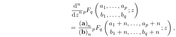
§16.3(i) Differentiation Formulas
►
16.3.1
…
►
16.3.3
…
►Two generalized hypergeometric functions are (generalized)
contiguous if they have the same pair of values of and , and corresponding parameters differ by integers.
…
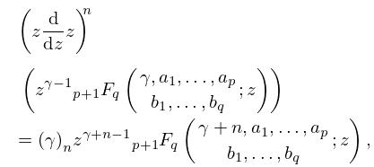
►
16.3.6
…
