Gauss%E2%80%93Christoffel%20quadrature

SearchAdvancedHelp

(0.003 seconds)

1—10 of 233 matching pages

1: 3.5 Quadrature

… ►

§3.5(v) Gauss Quadrature

… ►The remainder is given by … ►

Gauss–Legendre Formula

… ►

Gauss–Chebyshev Formula

… ►

Gauss–Laguerre Formula

…

2: 35.10 Methods of Computation

… ►Other methods include numerical quadrature applied to double and multiple integral representations. See Yan (1992) for the ${}_1{}^{}F_1^{}$ and ${}_2{}^{}F_1^{}$ functions of matrix argument in the case $m=2$, and Bingham et al. (1992) for Monte Carlo simulation on $𝐎(m)$ applied to a generalization of the integral (35.5.8). …

3: 15.5 Derivatives and Contiguous Functions

… ►The six functions $F(a\pm 1,b;c;z)$, $F(a,b\pm 1;c;z)$, $F(a,b;c\pm 1;z)$ are said to be contiguous to $F(a,b;c;z)$. ►

15.5.11 $$(c-a)F(a-1,b;c;z)+\left(2a-c+(b-a)z\right)F(a,b;c;z)+a(z-1)F(a+1,b;c;z)=0,$$

ⓘ

Symbols:

$F(a,b;c;z)$ or $F(\genfrac{}{}{0pt}{}{a,b}{c};z)$: $={}_2{}^{}F_1^{}(a,b;c;z)$ Gauss’ hypergeometric function, $z$: complex variable, $a$: real or complex parameter, $b$: real or complex parameter and $c$: real or complex parameter

Referenced by:

§15.4(i), §15.5(ii)

Permalink:

http://dlmf.nist.gov/15.5.E11

Encodings:

pMML, png, TeX

See also:

Annotations for §15.5(ii), §15.5 and Ch.15

►

15.5.12 $$(b-a)F(a,b;c;z)+aF(a+1,b;c;z)-bF(a,b+1;c;z)=0,$$

ⓘ

Symbols:

$F(a,b;c;z)$ or $F(\genfrac{}{}{0pt}{}{a,b}{c};z)$: $={}_2{}^{}F_1^{}(a,b;c;z)$ Gauss’ hypergeometric function, $z$: complex variable, $a$: real or complex parameter, $b$: real or complex parameter and $c$: real or complex parameter

Permalink:

http://dlmf.nist.gov/15.5.E12

Encodings:

pMML, png, TeX

See also:

Annotations for §15.5(ii), §15.5 and Ch.15

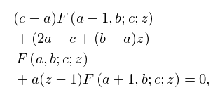
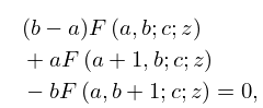
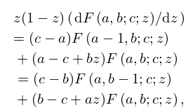
… ►By repeated applications of (15.5.11)–(15.5.18) any function $F(a+k,b+\mathrm{\ell };c+m;z)$, in which $k,\mathrm{\ell },m$ are integers, can be expressed as a linear combination of $F(a,b;c;z)$ and any one of its contiguous functions, with coefficients that are rational functions of $a,b,c$, and $z$. … ►

15.5.20 $$z(1-z)\left(dF(a,b;c;z)/dz\right)=(c-a)F(a-1,b;c;z)+(a-c+bz)F(a,b;c;z)=(c-b)F(a,b-1;c;z)+(b-c+az)F(a,b;c;z),$$

ⓘ

Symbols:

$F(a,b;c;z)$ or $F(\genfrac{}{}{0pt}{}{a,b}{c};z)$: $={}_2{}^{}F_1^{}(a,b;c;z)$ Gauss’ hypergeometric function, $\frac{df}{dx}$: derivative of $f$ with respect to $x$ , $z$: complex variable, $a$: real or complex parameter, $b$: real or complex parameter and $c$: real or complex parameter

Permalink:

http://dlmf.nist.gov/15.5.E20

Encodings:

pMML, png, TeX

See also:

Annotations for §15.5(ii), §15.5 and Ch.15

…

4: 20.11 Generalizations and Analogs

… ►

§20.11(i) Gauss Sum

►For relatively prime integers $m,n$ with $n>0$ and $mn$ even, the Gauss sum $G(m,n)$ is defined by … … ►

20.11.5 $${}_2{}^{}F_1^{}(\frac{1}{2},\frac{1}{2};1;k^2)={\theta }_3^2\left(0\right|\tau );$$

ⓘ

Symbols:

${}_2{}^{}F_1^{}(a,b;c;z)$: $=F(a,b;c;z)$ notation for Gauss’ hypergeometric function, ${\theta }_j\left(z\right|\tau )$: theta function, $\tau$: lattice parameter and $k$: modulus

Permalink:

http://dlmf.nist.gov/20.11.E5

Encodings:

pMML, png, TeX

See also:

Annotations for §20.11(iii), §20.11 and Ch.20

… ►Similar identities can be constructed for ${}_2{}^{}F_1^{}(\frac{1}{3},\frac{2}{3};1;k^2)$, ${}_2{}^{}F_1^{}(\frac{1}{4},\frac{3}{4};1;k^2)$, and ${}_2{}^{}F_1^{}(\frac{1}{6},\frac{5}{6};1;k^2)$. …

5: 15.19 Methods of Computation

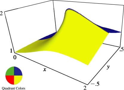
… ►The Gauss series (15.2.1) converges for . … ►Large values of $|a|$ or $|b|$, for example, delay convergence of the Gauss series, and may also lead to severe cancellation. ►For fast computation of $F(a,b;c;z)$ with $a,b$ and $c$ complex, and with application to Pöschl–Teller–Ginocchio potential wave functions, see Michel and Stoitsov (2008). … ►Gauss quadrature approximations are discussed in Gautschi (2002b). … ►For example, in the half-plane $\mathrm{\Re }z\le \frac{1}{2}$ we can use (15.12.2) or (15.12.3) to compute $F(a,b;c+N+1;z)$ and $F(a,b;c+N;z)$, where $N$ is a large positive integer, and then apply (15.5.18) in the backward direction. …

6: 18.5 Explicit Representations

… ►For the definitions of ${}_2{}^{}F_1^{}$, ${}_1{}^{}F_1^{}$, and ${}_2{}^{}F_0^{}$ see §16.2. … ►

18.5.9 $$C_n^{(\lambda )}\left(x\right)=\frac{{\left(2\lambda \right)}_n}{n!}{}_2{}^{}F_1^{}(\genfrac{}{}{0pt}{}{-n,n+2\lambda }{\lambda +\frac{1}{2}};\frac{1-x}{2}),$$

ⓘ

Symbols:

${}_2{}^{}F_1^{}(a,b;c;z)$: $=F(a,b;c;z)$ notation for Gauss’ hypergeometric function, ${\left(a\right)}_n$: Pochhammer’s symbol (or shifted factorial), $!$: factorial (as in $n!$), $C_n^{(\lambda )}\left(x\right)$: ultraspherical (or Gegenbauer) polynomial, $n$: nonnegative integer and $x$: real variable

A&S Ref:

22.5.46

Referenced by:

§18.5(iii), §18.6(i)

Permalink:

http://dlmf.nist.gov/18.5.E9

Encodings:

pMML, png, TeX

See also:

Annotations for §18.5(iii), §18.5(iii), §18.5 and Ch.18

… ►

18.5.11_1 $$T_n\left(x\right)=\frac{1}{2}n\sum _{\mathrm{\ell }=0}^{\lfloor n/2\rfloor }\frac{{(-1)}^{\mathrm{\ell }}(n-\mathrm{\ell }-1)!}{\mathrm{\ell }!(n-2\mathrm{\ell })!}{(2x)}^{n-2\mathrm{\ell }}=2^{n-1}{x}^n{}_2{}^{}F_1^{}(\genfrac{}{}{0pt}{}{-\frac{1}{2}n,-\frac{1}{2}n+\frac{1}{2}}{1-n};\frac{1}{x^2}),$$ $n\ge 1$,

ⓘ

Symbols:

$T_n\left(x\right)$: Chebyshev polynomial of the first kind, ${}_2{}^{}F_1^{}(a,b;c;z)$: $=F(a,b;c;z)$ notation for Gauss’ hypergeometric function, $!$: factorial (as in $n!$), $\lfloor x\rfloor$: floor of $x$ , $\mathrm{\ell }$: nonnegative integer, $n$: nonnegative integer and $x$: real variable

Source:

Erdélyi et al. (1953b, 10.11(22))

Referenced by:

§18.5(iii), Erratum (V1.2.0) Section 18.5

Permalink:

http://dlmf.nist.gov/18.5.E11_1

Encodings:

pMML, png, TeX

Addition (effective with 1.2.0):

This equation was added.

See also:

Annotations for §18.5(iii), §18.5(iii), §18.5 and Ch.18

►

18.5.11_2 $$T_n\left(x\right)={}_2{}^{}F_1^{}(\genfrac{}{}{0pt}{}{-n,n}{\frac{1}{2}};\frac{1-x}{2}),$$

ⓘ

Symbols:

$T_n\left(x\right)$: Chebyshev polynomial of the first kind, ${}_2{}^{}F_1^{}(a,b;c;z)$: $=F(a,b;c;z)$ notation for Gauss’ hypergeometric function, $n$: nonnegative integer and $x$: real variable

Permalink:

http://dlmf.nist.gov/18.5.E11_2

Encodings:

pMML, png, TeX

Addition (effective with 1.2.0):

This equation was added.

See also:

Annotations for §18.5(iii), §18.5(iii), §18.5 and Ch.18

… ►

18.5.11_4 $$U_n\left(x\right)=\left(n+1\right){}_2{}^{}F_1^{}(\genfrac{}{}{0pt}{}{-n,n+2}{\frac{3}{2}};\frac{1-x}{2}).$$

ⓘ

Symbols:

$U_n\left(x\right)$: Chebyshev polynomial of the second kind, ${}_2{}^{}F_1^{}(a,b;c;z)$: $=F(a,b;c;z)$ notation for Gauss’ hypergeometric function, $n$: nonnegative integer and $x$: real variable

Referenced by:

§18.5(iii), Erratum (V1.2.0) Section 18.5

Permalink:

http://dlmf.nist.gov/18.5.E11_4

Encodings:

pMML, png, TeX

Addition (effective with 1.2.0):

This equation was added.

See also:

Annotations for §18.5(iii), §18.5(iii), §18.5 and Ch.18

…

7: 27.2 Functions

… ►Euclid’s Elements (Euclid (1908, Book IX, Proposition 20)) gives an elegant proof that there are infinitely many primes. … ►Gauss and Legendre conjectured that $\pi \left(x\right)$ is asymptotic to $x/\ln x$ as $x\to \mathrm{\infty }$: …(See Gauss (1863, Band II, pp. 437–477) and Legendre (1808, p. 394).) … ►

Table 27.2.1: Primes.

► ►►

$n$	$p_n$	$p_{n+10}$	$p_{n+20}$	$p_{n+30}$	$p_{n+40}$	$p_{n+50}$	$p_{n+60}$	$p_{n+70}$	$p_{n+80}$	$p_{n+90}$
…

►

►

Table 27.2.2: Functions related to division.

► ►►►

$n$	$\varphi \left(n\right)$	$d\left(n\right)$	$\sigma \left(n\right)$	$n$	$\varphi \left(n\right)$	$d\left(n\right)$	$\sigma \left(n\right)$	$n$	$\varphi \left(n\right)$	$d\left(n\right)$	$\sigma \left(n\right)$	$n$	$\varphi \left(n\right)$	$d\left(n\right)$	$\sigma \left(n\right)$
…
11	10	2	12	24	8	8	60	37	36	2	38	50	20	6	93
…

►

8: 15.10 Hypergeometric Differential Equation

… ►

$f_1(z)=F({\displaystyle \genfrac{}{}{0pt}{}{a,b}{c}};z),$

… ►

$f_1(z)=F({\displaystyle \genfrac{}{}{0pt}{}{a,b}{a+b+1-c}};1-z),$

… ►(b) If $c$ equals $n=1,2,3,\mathrm{\dots }$, and $a\ne 1,2,\mathrm{\dots },n-1$, then fundamental solutions in the neighborhood of $z=0$ are given by $F(a,b;n;z)$ and … ►

15.10.11 $$w_1(z)=F(\genfrac{}{}{0pt}{}{a,b}{c};z)={(1-z)}^{c-a-b}F(\genfrac{}{}{0pt}{}{c-a,c-b}{c};z)={(1-z)}^{-a}F(\genfrac{}{}{0pt}{}{a,c-b}{c};\frac{z}{z-1})={(1-z)}^{-b}F(\genfrac{}{}{0pt}{}{c-a,b}{c};\frac{z}{z-1}).$$

ⓘ

Defines:

$w_1(z)$: Kummer’s solution $w_1$ (locally)

Symbols:

$F(a,b;c;z)$ or $F(\genfrac{}{}{0pt}{}{a,b}{c};z)$: $={}_2{}^{}F_1^{}(a,b;c;z)$ Gauss’ hypergeometric function, $z$: complex variable, $a$: real or complex parameter, $b$: real or complex parameter and $c$: real or complex parameter

Permalink:

http://dlmf.nist.gov/15.10.E11

Encodings:

pMML, png, TeX

See also:

Annotations for §15.10(ii), §15.10 and Ch.15

… ►The $\left(\genfrac{}{}{0.0pt}{}{6}{3}\right)=20$ connection formulas for the principal branches of Kummer’s solutions are: …

9: 15.3 Graphics

… ►

►►

Figure 15.3.1: $F(\frac{4}{3},\frac{9}{16};\frac{14}{5};x),-100\le x\le 1$. Magnify

►

►►

Figure 15.3.2: $F(5,-10;1;x),-0.023\le x\le 1$. Magnify

►

►►

Figure 15.3.3: $F(1,-10;10;x),-3\le x\le 1$. Magnify

►

►►

Figure 15.3.4: $F(5,10;1;x),-1\le x\le 0.022$. Magnify

… ►

►

►

Figure 15.3.5: $F(\frac{4}{3},\frac{9}{16};\frac{14}{5};x+\mathrm{i}y),0\le x\le 2,-0.5\le y\le 0.5$. … Magnify 3D Help

…

10: 16.12 Products

… ►

16.12.1 $${}_0{}^{}F_1^{}(-;a;z){}_0{}^{}F_1^{}(-;b;z)={}_2{}^{}F_3^{}(\genfrac{}{}{0pt}{}{\frac{1}{2}(a+b),\frac{1}{2}(a+b-1)}{a,b,a+b-1};4z).$$

ⓘ

Symbols:

${}_p{}^{}F_q^{}(a_1,\mathrm{\dots },a_p;b_1,\mathrm{\dots },b_q;z)$ or ${}_p{}^{}F_q^{}(\genfrac{}{}{0pt}{}{a_1,\mathrm{\dots },a_p}{b_1,\mathrm{\dots },b_q};z)$: alternatively ${}_p{}^{}F_q^{}(𝐚;𝐛;z)$ or ${}_p{}^{}F_q^{}(\genfrac{}{}{0pt}{}{𝐚}{𝐛};z)$
generalized hypergeometric function, $z$: complex variable, $a,a_1,\mathrm{\dots },a_p$: real or complex parameters and $b,b_1,\mathrm{\dots },b_q$: real or complex parameters

Referenced by:

(10.8.3), §10.8, §10.8, §16.12, Erratum (V1.0.17) for Section 10.8

Permalink:

http://dlmf.nist.gov/16.12.E1

Encodings:

pMML, png, TeX

See also:

Annotations for §16.12 and Ch.16

… ►

16.12.2 $${\left({}_2{}^{}F_1^{}(\genfrac{}{}{0pt}{}{a,b}{a+b+\frac{1}{2}};z)\right)}^2={}_3{}^{}F_2^{}(\genfrac{}{}{0pt}{}{2a,2b,a+b}{a+b+\frac{1}{2},2a+2b};z).$$

ⓘ

Symbols:

${}_2{}^{}F_1^{}(a,b;c;z)$: $=F(a,b;c;z)$ notation for Gauss’ hypergeometric function, ${}_p{}^{}F_q^{}(a_1,\mathrm{\dots },a_p;b_1,\mathrm{\dots },b_q;z)$ or ${}_p{}^{}F_q^{}(\genfrac{}{}{0pt}{}{a_1,\mathrm{\dots },a_p}{b_1,\mathrm{\dots },b_q};z)$: alternatively ${}_p{}^{}F_q^{}(𝐚;𝐛;z)$ or ${}_p{}^{}F_q^{}(\genfrac{}{}{0pt}{}{𝐚}{𝐛};z)$
generalized hypergeometric function, $z$: complex variable, $a,a_1,\mathrm{\dots },a_p$: real or complex parameters and $b,b_1,\mathrm{\dots },b_q$: real or complex parameters

Referenced by:

§16.12, §17.9(iii), Erratum (V1.1.12) for Subsection 17.9(iii)

Permalink:

http://dlmf.nist.gov/16.12.E2

Encodings:

pMML, png, TeX

See also:

Annotations for §16.12 and Ch.16

… ►

16.12.3 $${\left({}_2{}^{}F_1^{}(\genfrac{}{}{0pt}{}{a,b}{c};z)\right)}^2=\sum _{k=0}^{\mathrm{\infty }}\frac{{\left(2a\right)}_k{\left(2b\right)}_k{\left(c-\frac{1}{2}\right)}_k}{{\left(c\right)}_k{\left(2c-1\right)}_{k}k!}{}_4{}^{}F_3^{}(\genfrac{}{}{0pt}{}{-\frac{1}{2}k,\frac{1}{2}(1-k),a+b-c+\frac{1}{2},\frac{1}{2}}{a+\frac{1}{2},b+\frac{1}{2},\frac{3}{2}-k-c};1)z^k,$$ .

ⓘ

Symbols:

${}_2{}^{}F_1^{}(a,b;c;z)$: $=F(a,b;c;z)$ notation for Gauss’ hypergeometric function, ${}_p{}^{}F_q^{}(a_1,\mathrm{\dots },a_p;b_1,\mathrm{\dots },b_q;z)$ or ${}_p{}^{}F_q^{}(\genfrac{}{}{0pt}{}{a_1,\mathrm{\dots },a_p}{b_1,\mathrm{\dots },b_q};z)$: alternatively ${}_p{}^{}F_q^{}(𝐚;𝐛;z)$ or ${}_p{}^{}F_q^{}(\genfrac{}{}{0pt}{}{𝐚}{𝐛};z)$
generalized hypergeometric function, ${\left(a\right)}_n$: Pochhammer’s symbol (or shifted factorial), $!$: factorial (as in $n!$), $z$: complex variable, $a,a_1,\mathrm{\dots },a_p$: real or complex parameters and $b,b_1,\mathrm{\dots },b_q$: real or complex parameters

Referenced by:

§16.12

Permalink:

http://dlmf.nist.gov/16.12.E3

Encodings:

pMML, png, TeX

See also:

Annotations for §16.12 and Ch.16

…