Fourier coefficients

SearchAdvancedHelp

(0.002 seconds)

11—20 of 39 matching pages

11: 28.34 Methods of Computation

… ►

Solution of the systems of linear algebraic equations (28.4.5)–(28.4.8) and (28.14.4), with the conditions (28.4.9)–(28.4.12) and (28.14.5), by boundary-value methods (§3.6) to determine the Fourier coefficients. Subsequently, the Fourier series can be summed with the aid of Clenshaw’s algorithm (§3.11(ii)). See Meixner and Schäfke (1954, §2.87). This procedure can be combined with §28.34(ii)(d).

…

12: 28.22 Connection Formulas

… ►

28.22.5 $$g_{e,2m}(h)={(-1)}^m\sqrt{\frac{2}{\pi }}\frac{{\mathrm{ce}}_{2m}(\frac{1}{2}\pi ,h^2)}{A_0^{2m}(h^2)},$$

ⓘ

Symbols:

${\mathrm{ce}}_n(z,q)$: Mathieu function, $\pi$: the ratio of the circumference of a circle to its diameter, $m$: integer, $h$: parameter, $g_{e,n}(h)$, $g_{o,n}(h)$: joining factors and $A_m(q)$: Fourier coefficient

Permalink:

http://dlmf.nist.gov/28.22.E5

Encodings:

pMML, png, TeX

See also:

Annotations for §28.22(i), §28.22 and Ch.28

►

28.22.6 $$g_{e,2m+1}(h)={(-1)}^{m+1}\sqrt{\frac{2}{\pi }}\frac{{\mathrm{ce}}_{2m+1}^{\prime }(\frac{1}{2}\pi ,h^2)}{h{A}_1^{2m+1}(h^2)},$$

ⓘ

Symbols:

${\mathrm{ce}}_n(z,q)$: Mathieu function, $\pi$: the ratio of the circumference of a circle to its diameter, $m$: integer, $h$: parameter, $g_{e,n}(h)$, $g_{o,n}(h)$: joining factors and $A_m(q)$: Fourier coefficient

Permalink:

http://dlmf.nist.gov/28.22.E6

Encodings:

pMML, png, TeX

See also:

Annotations for §28.22(i), §28.22 and Ch.28

►

28.22.7 $$g_{o,2m+1}(h)={(-1)}^m\sqrt{\frac{2}{\pi }}\frac{{\mathrm{se}}_{2m+1}(\frac{1}{2}\pi ,h^2)}{h{B}_1^{2m+1}(h^2)},$$

ⓘ

Symbols:

${\mathrm{se}}_n(z,q)$: Mathieu function, $\pi$: the ratio of the circumference of a circle to its diameter, $m$: integer, $h$: parameter, $g_{e,n}(h)$, $g_{o,n}(h)$: joining factors and $B_m(q)$: Fourier coefficient

Permalink:

http://dlmf.nist.gov/28.22.E7

Encodings:

pMML, png, TeX

See also:

Annotations for §28.22(i), §28.22 and Ch.28

►

28.22.8 $$g_{o,2m+2}(h)={(-1)}^{m+1}\sqrt{\frac{2}{\pi }}\frac{{\mathrm{se}}_{2m+2}^{\prime }(\frac{1}{2}\pi ,h^2)}{h^2{B}_2^{2m+2}(h^2)},$$

ⓘ

Symbols:

${\mathrm{se}}_n(z,q)$: Mathieu function, $\pi$: the ratio of the circumference of a circle to its diameter, $m$: integer, $h$: parameter, $g_{e,n}(h)$, $g_{o,n}(h)$: joining factors and $B_m(q)$: Fourier coefficient

Permalink:

http://dlmf.nist.gov/28.22.E8

Encodings:

pMML, png, TeX

See also:

Annotations for §28.22(i), §28.22 and Ch.28

…

13: 1.8 Fourier Series

… ►The series (1.8.1) is called the Fourier series of $f(x)$, and $a_n,b_n$ are the Fourier coefficients of $f(x)$. … ►If $g(x)$ is also square-integrable with Fourier coefficients $a_n^{\prime },b_n^{\prime }$ or $c_n^{\prime }$ then … ►If $f(x)$ and $g(x)$ are continuous, have the same period and same Fourier coefficients, then $f(x)=g(x)$ for all $x$. … ►If $a_n$ and $b_n$ are the Fourier coefficients of a piecewise continuous function $f(x)$ on $[0,2\pi ]$, then …

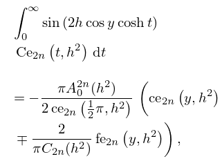
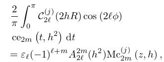
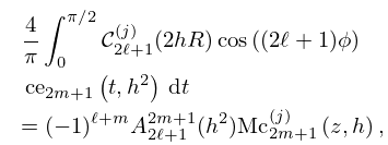
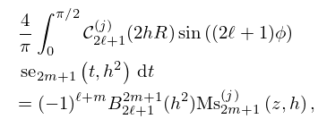
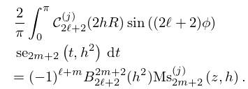
14: 28.28 Integrals, Integral Representations, and Integral Equations

… ►

28.28.16 $${\int }_0^{\mathrm{\infty }}\sin \left(2h\cos y\cosh t\right){\mathrm{Ce}}_{2n}(t,h^2)dt=-\frac{\pi A_0^{2n}(h^2)}{2{\mathrm{ce}}_{2n}(\frac{1}{2}\pi ,h^2)}\left({\mathrm{ce}}_{2n}(y,h^2)\mp \frac{2}{\pi C_{2n}(h^2)}{\mathrm{fe}}_{2n}(y,h^2)\right),$$

ⓘ

Symbols:

${\mathrm{ce}}_n(z,q)$: Mathieu function, ${\mathrm{fe}}_n(z,q)$: second solution, Mathieu’s equation, $\pi$: the ratio of the circumference of a circle to its diameter, $\cos z$: cosine function, $dx$: differential of $x$ , $\cosh z$: hyperbolic cosine function, $\int$: integral, ${\mathrm{Ce}}_{\nu }(z,q)$: modified Mathieu function, $\sin z$: sine function, $h$: parameter, $n$: integer, $y$: real variable, $A_m(q)$: Fourier coefficient and $C_n(q)$: factor

Permalink:

http://dlmf.nist.gov/28.28.E16

Encodings:

pMML, png, TeX

See also:

Annotations for §28.28(i), §28.28 and Ch.28

… ►

28.28.20 $$\frac{2}{\pi }{\int }_0^{\pi }{𝒞}_{2\mathrm{\ell }}^{(j)}(2hR)\cos \left(2\mathrm{\ell }\varphi \right){\mathrm{ce}}_{2m}(t,h^2)dt={\epsilon }_{\mathrm{\ell }}{(-1)}^{\mathrm{\ell }+m}{A}_{2\mathrm{\ell }}^{2m}(h^2){\mathrm{Mc}}_{2m}^{(j)}(z,h),$$

ⓘ

Symbols:

${\mathrm{ce}}_n(z,q)$: Mathieu function, $\pi$: the ratio of the circumference of a circle to its diameter, $\cos z$: cosine function, $dx$: differential of $x$ , $\int$: integral, ${\mathrm{Mc}}_n^{(j)}(z,h)$: radial Mathieu function, $m$: integer, $h$: parameter, $j$: integer, $z$: complex variable, ${𝒞}_{\mu }^{(j)}$: cylinder functions, $\varphi (z,t)$: function, $R(z,t)$: function, ${\epsilon }_{\mathrm{\ell }}$: constants and $A_m(q)$: Fourier coefficient

A&S Ref:

20.7.26 (in different form and only for $\mathrm{\ell }=0$)

Permalink:

http://dlmf.nist.gov/28.28.E20

Encodings:

pMML, png, TeX

See also:

Annotations for §28.28(ii), §28.28 and Ch.28

… ►

28.28.21 $$\frac{4}{\pi }{\int }_0^{\pi /2}{𝒞}_{2\mathrm{\ell }+1}^{(j)}(2hR)\cos \left((2\mathrm{\ell }+1)\varphi \right){\mathrm{ce}}_{2m+1}(t,h^2)dt={(-1)}^{\mathrm{\ell }+m}{A}_{2\mathrm{\ell }+1}^{2m+1}(h^2){\mathrm{Mc}}_{2m+1}^{(j)}(z,h),$$

ⓘ

Symbols:

${\mathrm{ce}}_n(z,q)$: Mathieu function, $\pi$: the ratio of the circumference of a circle to its diameter, $\cos z$: cosine function, $dx$: differential of $x$ , $\int$: integral, ${\mathrm{Mc}}_n^{(j)}(z,h)$: radial Mathieu function, $m$: integer, $h$: parameter, $j$: integer, $z$: complex variable, ${𝒞}_{\mu }^{(j)}$: cylinder functions, $\varphi (z,t)$: function, $R(z,t)$: function and $A_m(q)$: Fourier coefficient

A&S Ref:

20.7.26 (in different form and only for $\mathrm{\ell }=0$)

Referenced by:

Erratum (V1.0.11) for Equations (28.28.21) and (28.28.22)

Permalink:

http://dlmf.nist.gov/28.28.E21

Encodings:

pMML, png, TeX

Errata (effective with 1.0.11):

Originally the prefactor and uppper limit of integration were given incorrectly as ${\displaystyle \frac{2}{\pi }}{\int }_0^{\pi }$.

Reported 2015-05-20 by Ruslan Kabasayev

See also:

Annotations for §28.28(ii), §28.28 and Ch.28

►

28.28.22 $$\frac{4}{\pi }{\int }_0^{\pi /2}{𝒞}_{2\mathrm{\ell }+1}^{(j)}(2hR)\sin \left((2\mathrm{\ell }+1)\varphi \right){\mathrm{se}}_{2m+1}(t,h^2)dt={(-1)}^{\mathrm{\ell }+m}{B}_{2\mathrm{\ell }+1}^{2m+1}(h^2){\mathrm{Ms}}_{2m+1}^{(j)}(z,h),$$

ⓘ

Symbols:

${\mathrm{se}}_n(z,q)$: Mathieu function, $\pi$: the ratio of the circumference of a circle to its diameter, $dx$: differential of $x$ , $\int$: integral, ${\mathrm{Ms}}_n^{(j)}(z,h)$: radial Mathieu function, $\sin z$: sine function, $m$: integer, $h$: parameter, $j$: integer, $z$: complex variable, ${𝒞}_{\mu }^{(j)}$: cylinder functions, $\varphi (z,t)$: function, $R(z,t)$: function and $B_m(q)$: Fourier coefficient

A&S Ref:

20.7.27 (in different form and only for $\mathrm{\ell }=0$)

Referenced by:

Erratum (V1.0.11) for Equations (28.28.21) and (28.28.22)

Permalink:

http://dlmf.nist.gov/28.28.E22

Encodings:

pMML, png, TeX

Errata (effective with 1.0.11):

Originally the prefactor and uppper limit of integration were given incorrectly as ${\displaystyle \frac{2}{\pi }}{\int }_0^{\pi }$.

Reported 2015-05-20 by Ruslan Kabasayev

See also:

Annotations for §28.28(ii), §28.28 and Ch.28

►

28.28.23 $$\frac{2}{\pi }{\int }_0^{\pi }{𝒞}_{2\mathrm{\ell }+2}^{(j)}(2hR)\sin \left((2\mathrm{\ell }+2)\varphi \right){\mathrm{se}}_{2m+2}(t,h^2)dt={(-1)}^{\mathrm{\ell }+m}{B}_{2\mathrm{\ell }+2}^{2m+2}(h^2){\mathrm{Ms}}_{2m+2}^{(j)}(z,h).$$

ⓘ

Symbols:

${\mathrm{se}}_n(z,q)$: Mathieu function, $\pi$: the ratio of the circumference of a circle to its diameter, $dx$: differential of $x$ , $\int$: integral, ${\mathrm{Ms}}_n^{(j)}(z,h)$: radial Mathieu function, $\sin z$: sine function, $m$: integer, $h$: parameter, $j$: integer, $z$: complex variable, ${𝒞}_{\mu }^{(j)}$: cylinder functions, $\varphi (z,t)$: function, $R(z,t)$: function and $B_m(q)$: Fourier coefficient

A&S Ref:

20.7.28 (in different form and only for $\mathrm{\ell }=0$)

Permalink:

http://dlmf.nist.gov/28.28.E23

Encodings:

pMML, png, TeX

See also:

Annotations for §28.28(ii), §28.28 and Ch.28

…

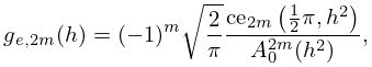
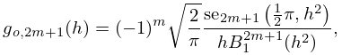
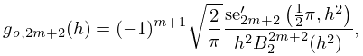
15: 29.15 Fourier Series and Chebyshev Series

… ►

§29.15(i) Fourier Coefficients

…

16: Bibliography W

… ►

On the asymptotic behavior of the Fourier coefficients of Mathieu functions. J. Res. Nat. Inst. Standards Tech. 113 (1), pp. 11–15.

ⓘ

External Links:

ISSN 1044-677X, FullText

Referenced by:

§28.4(vii).

Encodings:

BibTeX

…

17: 28.29 Definitions and Basic Properties

… ►For this purpose the discriminant can be expressed as an infinite determinant involving the Fourier coefficients of $Q(x)$; see Magnus and Winkler (1966, §2.3, pp. 28–36). …

18: Bibliography L

… ►

Adjusted forms of the Fourier coefficient asymptotic expansion and applications in numerical quadrature. Math. Comp. 25 (113), pp. 87–104.

ⓘ

External Links:

FullText, MathReview (J. Bryant), ZentralBlatt

Referenced by:

§2.3(iv).

Encodings:

BibTeX

…

19: 28.31 Equations of Whittaker–Hill and Ince

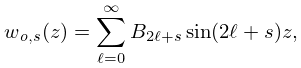
… ►Formal $2\pi$-periodic solutions can be constructed as Fourier series; compare §28.4: … ►

28.31.5 $$w_{o,s}(z)=\sum _{\mathrm{\ell }=0}^{\mathrm{\infty }}{B}_{2\mathrm{\ell }+s}\sin (2\mathrm{\ell }+s)z,$$ $s=1,2$,

ⓘ

Symbols:

$\sin z$: sine function, $z$: complex variable, $w(z)$: Mathieu’s equation solution and $B$: constant

Referenced by:

§28.31(ii)

Permalink:

http://dlmf.nist.gov/28.31.E5

Encodings:

pMML, png, TeX

See also:

Annotations for §28.31(ii), §28.31 and Ch.28

►where the coefficients satisfy …

20: 28.2 Definitions and Basic Properties

… ►

28.2.18 $$w(z)=\sum _{n=-\mathrm{\infty }}^{\mathrm{\infty }}{c}_{2n}{\mathrm{e}}^{\mathrm{i}(\nu +2n)z}$$

ⓘ

Symbols:

$\mathrm{e}$: base of natural logarithm, $\mathrm{i}$: imaginary unit, $n$: integer, $z$: complex variable, $\nu$: complex parameter, $w(z)$: Mathieu’s equation solution and $c_{2n}$: coefficients

A&S Ref:

20.3.8

Permalink:

http://dlmf.nist.gov/28.2.E18

Encodings:

pMML, png, TeX

See also:

Annotations for §28.2(iv), §28.2 and Ch.28

…