Fourier coefficients

SearchAdvancedHelp

(0.002 seconds)

1—10 of 39 matching pages

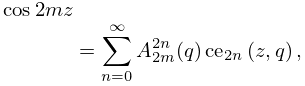
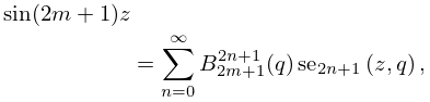
1: 28.4 Fourier Series

… ►

§28.4(ii) Recurrence Relations

… ►

§28.4(iii) Normalization

… ►

§28.4(v) Change of Sign of $q$

… ►

§28.4(vi) Behavior for Small $q$

… ►

§28.4(vii) Asymptotic Forms for Large $m$

…

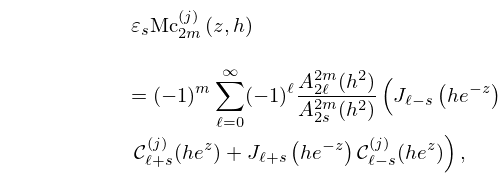
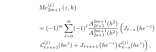
2: 28.11 Expansions in Series of Mathieu Functions

… ►

28.11.3 $$1=2\sum _{n=0}^{\mathrm{\infty }}{A}_0^{2n}(q){\mathrm{ce}}_{2n}(z,q),$$

ⓘ

Symbols:

${\mathrm{ce}}_n(z,q)$: Mathieu function, $q=h^2$: parameter, $n$: integer, $z$: complex variable and $A_m(q)$: Fourier coefficient

Permalink:

http://dlmf.nist.gov/28.11.E3

Encodings:

pMML, png, TeX

See also:

Annotations for §28.11, §28.11 and Ch.28

►

28.11.4 $$\cos 2mz=\sum _{n=0}^{\mathrm{\infty }}{A}_{2m}^{2n}(q){\mathrm{ce}}_{2n}(z,q),$$ $m\ne 0$,

ⓘ

Symbols:

${\mathrm{ce}}_n(z,q)$: Mathieu function, $\cos z$: cosine function, $m$: integer, $q=h^2$: parameter, $n$: integer, $z$: complex variable and $A_m(q)$: Fourier coefficient

Permalink:

http://dlmf.nist.gov/28.11.E4

Encodings:

pMML, png, TeX

See also:

Annotations for §28.11, §28.11 and Ch.28

►

28.11.5 $$\cos (2m+1)z=\sum _{n=0}^{\mathrm{\infty }}{A}_{2m+1}^{2n+1}(q){\mathrm{ce}}_{2n+1}(z,q),$$

ⓘ

Symbols:

${\mathrm{ce}}_n(z,q)$: Mathieu function, $\cos z$: cosine function, $m$: integer, $q=h^2$: parameter, $n$: integer, $z$: complex variable and $A_m(q)$: Fourier coefficient

Permalink:

http://dlmf.nist.gov/28.11.E5

Encodings:

pMML, png, TeX

See also:

Annotations for §28.11, §28.11 and Ch.28

►

28.11.6 $$\sin (2m+1)z=\sum _{n=0}^{\mathrm{\infty }}{B}_{2m+1}^{2n+1}(q){\mathrm{se}}_{2n+1}(z,q),$$

ⓘ

Symbols:

${\mathrm{se}}_n(z,q)$: Mathieu function, $\sin z$: sine function, $m$: integer, $q=h^2$: parameter, $n$: integer, $z$: complex variable and $B_m(q)$: Fourier coefficient

Permalink:

http://dlmf.nist.gov/28.11.E6

Encodings:

pMML, png, TeX

See also:

Annotations for §28.11, §28.11 and Ch.28

►

28.11.7 $$\sin (2m+2)z=\sum _{n=0}^{\mathrm{\infty }}{B}_{2m+2}^{2n+2}(q){\mathrm{se}}_{2n+2}(z,q).$$

ⓘ

Symbols:

${\mathrm{se}}_n(z,q)$: Mathieu function, $\sin z$: sine function, $m$: integer, $q=h^2$: parameter, $n$: integer, $z$: complex variable and $B_m(q)$: Fourier coefficient

Permalink:

http://dlmf.nist.gov/28.11.E7

Encodings:

pMML, png, TeX

See also:

Annotations for §28.11, §28.11 and Ch.28

3: 28.35 Tables

§28.35 Tables

… ►

Ince (1932) includes eigenvalues $a_n$, $b_n$, and Fourier coefficients for $n=0$ or $1(1)6$, $q=0(1)10(2)20(4)40$; 7D. Also ${\mathrm{ce}}_n(x,q)$, ${\mathrm{se}}_n(x,q)$ for $q=0(1)10$, $x=1(1)90$, corresponding to the eigenvalues in the tables; 5D. Notation: $a_n={\mathrm{𝑏𝑒}}_n-2q$, $b_n={\mathrm{𝑏𝑜}}_n-2q$.

… ►

National Bureau of Standards (1967) includes the eigenvalues $a_n\left(q\right)$, $b_n\left(q\right)$ for $n=0(1)3$ with $q=0(.2)20(.5)37(1)100$, and $n=4(1)15$ with $q=0(2)100$; Fourier coefficients for ${\mathrm{ce}}_n(x,q)$ and ${\mathrm{se}}_n(x,q)$ for $n=0(1)15$, $n=1(1)15$, respectively, and various values of $q$ in the interval $[0,100]$; joining factors $g_{e,n}(\sqrt{q})$, $f_{e,n}(\sqrt{q})$ for $n=0(1)15$ with $q=0(.5\text{ to }10)100$ (but in a different notation). Also, eigenvalues for large values of $q$. Precision is generally 8D.

►

Stratton et al. (1941) includes $b_n$, $b_n^{\prime }$, and the corresponding Fourier coefficients for ${\mathrm{Se}}_n(c,x)$ and ${\mathrm{So}}_n(c,x)$ for $n=0$ or $1(1)4$, $c=0(.1\text{or}.2)4.5$. Precision is mostly 5S. Notation: $c=2\sqrt{q}$, $b_n=a_n+2q$, $b_n^{\prime }=b_n+2q$, and for ${\mathrm{Se}}_n(c,x)$, ${\mathrm{So}}_n(c,x)$ see §28.1.

… ►

Blanch and Clemm (1969) includes eigenvalues $a_n\left(q\right)$, $b_n\left(q\right)$ for $q=\rho {\mathrm{e}}^{\mathrm{i}\varphi }$, $\rho =0(.5)25$, $\varphi =5^{\circ }(5^{\circ }){90}^{\circ }$, $n=0(1)15$; 4D. Also $a_n\left(q\right)$ and $b_n\left(q\right)$ for $q=\mathrm{i}\rho$, $\rho =0(.5)100$, $n=0(2)14$ and $n=2(2)16$, respectively; 8D. Double points for $n=0(1)15$; 8D. Graphs are included.

…

4: 28.14 Fourier Series

… ►

28.14.4 $$q{c}_{2m+2}-\left(a-{(\nu +2m)}^2\right)c_{2m}+q{c}_{2m-2}=0,$$ $a={\lambda }_{\nu }\left(q\right),c_{2m}=c_{2m}^{\nu }(q)$,

ⓘ

Symbols:

${\lambda }_{\nu +2n}\left(q\right)$: eigenvalues of Mathieu equation, $m$: integer, $q=h^2$: parameter, $\nu$: complex parameter, $a$: parameter and $c_{2m}(q)$: coefficients

Referenced by:

item (d), item (d)

Permalink:

http://dlmf.nist.gov/28.14.E4

Encodings:

pMML, png, TeX

See also:

Annotations for §28.14 and Ch.28

… ►

28.14.5 $$\sum _{m=-\mathrm{\infty }}^{\mathrm{\infty }}{\left(c_{2m}^{\nu }(q)\right)}^2=1;$$

ⓘ

Symbols:

$m$: integer, $q=h^2$: parameter, $\nu$: complex parameter and $c_{2m}(q)$: coefficients

Referenced by:

item (d)

Permalink:

http://dlmf.nist.gov/28.14.E5

Encodings:

pMML, png, TeX

See also:

Annotations for §28.14 and Ch.28

…

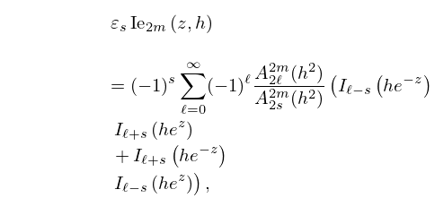
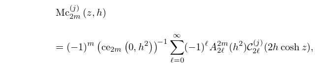
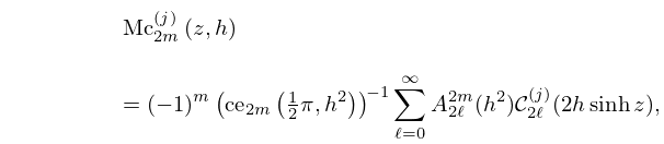
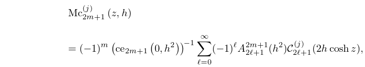
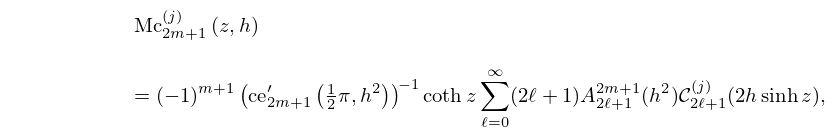
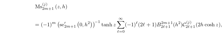
5: 28.24 Expansions in Series of Cross-Products of Bessel Functions or Modified Bessel Functions

… ►

28.24.2 $${\epsilon }_s{\mathrm{Mc}}_{2m}^{(j)}(z,h)={(-1)}^m\sum _{\mathrm{\ell }=0}^{\mathrm{\infty }}{(-1)}^{\mathrm{\ell }}\frac{A_{2\mathrm{\ell }}^{2m}(h^2)}{A_{2s}^{2m}(h^2)}\left(J_{\mathrm{\ell }-s}\left(h{\mathrm{e}}^{-z}\right){𝒞}_{\mathrm{\ell }+s}^{(j)}(h{\mathrm{e}}^z)+J_{\mathrm{\ell }+s}\left(h{\mathrm{e}}^{-z}\right){𝒞}_{\mathrm{\ell }-s}^{(j)}(h{\mathrm{e}}^z)\right),$$

ⓘ

Symbols:

$J_{\nu }\left(z\right)$: Bessel function of the first kind, $\mathrm{e}$: base of natural logarithm, ${\mathrm{Mc}}_n^{(j)}(z,h)$: radial Mathieu function, $m$: integer, $h$: parameter, $j$: integer, $z$: complex variable, ${𝒞}_{\mu }^{(j)}$: cylinder functions, ${\epsilon }_s$: constants and $A_m(q)$: Fourier coefficient

A&S Ref:

20.6.7

Permalink:

http://dlmf.nist.gov/28.24.E2

Encodings:

pMML, png, TeX

See also:

Annotations for §28.24 and Ch.28

►

28.24.3 $${\mathrm{Mc}}_{2m+1}^{(j)}(z,h)={(-1)}^m\sum _{\mathrm{\ell }=0}^{\mathrm{\infty }}{(-1)}^{\mathrm{\ell }}\frac{A_{2\mathrm{\ell }+1}^{2m+1}(h^2)}{A_{2s+1}^{2m+1}(h^2)}\left(J_{\mathrm{\ell }-s}\left(h{\mathrm{e}}^{-z}\right){𝒞}_{\mathrm{\ell }+s+1}^{(j)}(h{\mathrm{e}}^z)+J_{\mathrm{\ell }+s+1}\left(h{\mathrm{e}}^{-z}\right){𝒞}_{\mathrm{\ell }-s}^{(j)}(h{\mathrm{e}}^z)\right),$$

ⓘ

Symbols:

$J_{\nu }\left(z\right)$: Bessel function of the first kind, $\mathrm{e}$: base of natural logarithm, ${\mathrm{Mc}}_n^{(j)}(z,h)$: radial Mathieu function, $m$: integer, $h$: parameter, $j$: integer, $z$: complex variable, ${𝒞}_{\mu }^{(j)}$: cylinder functions and $A_m(q)$: Fourier coefficient

A&S Ref:

20.6.8

Permalink:

http://dlmf.nist.gov/28.24.E3

Encodings:

pMML, png, TeX

See also:

Annotations for §28.24 and Ch.28

►

28.24.4 $${\mathrm{Ms}}_{2m+1}^{(j)}(z,h)={(-1)}^m\sum _{\mathrm{\ell }=0}^{\mathrm{\infty }}{(-1)}^{\mathrm{\ell }}\frac{B_{2\mathrm{\ell }+1}^{2m+1}(h^2)}{B_{2s+1}^{2m+1}(h^2)}\left(J_{\mathrm{\ell }-s}\left(h{\mathrm{e}}^{-z}\right){𝒞}_{\mathrm{\ell }+s+1}^{(j)}(h{\mathrm{e}}^z)-J_{\mathrm{\ell }+s+1}\left(h{\mathrm{e}}^{-z}\right){𝒞}_{\mathrm{\ell }-s}^{(j)}(h{\mathrm{e}}^z)\right),$$

ⓘ

Symbols:

$J_{\nu }\left(z\right)$: Bessel function of the first kind, $\mathrm{e}$: base of natural logarithm, ${\mathrm{Ms}}_n^{(j)}(z,h)$: radial Mathieu function, $m$: integer, $h$: parameter, $j$: integer, $z$: complex variable, ${𝒞}_{\mu }^{(j)}$: cylinder functions and $B_m(q)$: Fourier coefficient

A&S Ref:

20.6.9

Permalink:

http://dlmf.nist.gov/28.24.E4

Encodings:

pMML, png, TeX

See also:

Annotations for §28.24 and Ch.28

►

28.24.5 $${\mathrm{Ms}}_{2m+2}^{(j)}(z,h)={(-1)}^m\sum _{\mathrm{\ell }=0}^{\mathrm{\infty }}{(-1)}^{\mathrm{\ell }}\frac{B_{2\mathrm{\ell }+2}^{2m+2}(h^2)}{B_{2s+2}^{2m+2}(h^2)}\left(J_{\mathrm{\ell }-s}\left(h{\mathrm{e}}^{-z}\right){𝒞}_{\mathrm{\ell }+s+2}^{(j)}(h{\mathrm{e}}^z)-J_{\mathrm{\ell }+s+2}\left(h{\mathrm{e}}^{-z}\right){𝒞}_{\mathrm{\ell }-s}^{(j)}(h{\mathrm{e}}^z)\right),$$

ⓘ

Symbols:

$J_{\nu }\left(z\right)$: Bessel function of the first kind, $\mathrm{e}$: base of natural logarithm, ${\mathrm{Ms}}_n^{(j)}(z,h)$: radial Mathieu function, $m$: integer, $h$: parameter, $j$: integer, $z$: complex variable, ${𝒞}_{\mu }^{(j)}$: cylinder functions and $B_m(q)$: Fourier coefficient

A&S Ref:

20.6.10

Permalink:

http://dlmf.nist.gov/28.24.E5

Encodings:

pMML, png, TeX

See also:

Annotations for §28.24 and Ch.28

… ►

28.24.6 $${\epsilon }_s{\mathrm{Ie}}_{2m}(z,h)={(-1)}^s\sum _{\mathrm{\ell }=0}^{\mathrm{\infty }}{(-1)}^{\mathrm{\ell }}\frac{A_{2\mathrm{\ell }}^{2m}(h^2)}{A_{2s}^{2m}(h^2)}\left(I_{\mathrm{\ell }-s}\left(h{\mathrm{e}}^{-z}\right)I_{\mathrm{\ell }+s}\left(h{\mathrm{e}}^z\right)+I_{\mathrm{\ell }+s}\left(h{\mathrm{e}}^{-z}\right)I_{\mathrm{\ell }-s}\left(h{\mathrm{e}}^z\right)\right),$$

ⓘ

Symbols:

$\mathrm{e}$: base of natural logarithm, $I_{\nu }\left(z\right)$: modified Bessel function of the first kind, ${\mathrm{Ie}}_n(z,h)$: modified Mathieu function, $m$: integer, $h$: parameter, $z$: complex variable, ${\epsilon }_s$: constants and $A_m(q)$: Fourier coefficient

A&S Ref:

20.8.8

Permalink:

http://dlmf.nist.gov/28.24.E6

Encodings:

pMML, png, TeX

See also:

Annotations for §28.24 and Ch.28

…

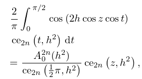
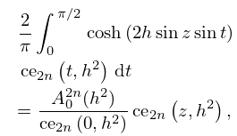
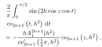
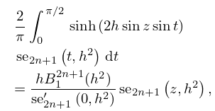
6: 28.10 Integral Equations

… ►With the notation of §28.4 for Fourier coefficients, ►

28.10.1 $$\frac{2}{\pi }{\int }_0^{\pi /2}\cos \left(2h\cos z\cos t\right){\mathrm{ce}}_{2n}(t,h^2)dt=\frac{A_0^{2n}(h^2)}{{\mathrm{ce}}_{2n}(\frac{1}{2}\pi ,h^2)}{\mathrm{ce}}_{2n}(z,h^2),$$

ⓘ

Symbols:

${\mathrm{ce}}_n(z,q)$: Mathieu function, $\pi$: the ratio of the circumference of a circle to its diameter, $\cos z$: cosine function, $dx$: differential of $x$ , $\int$: integral, $h$: parameter, $n$: integer, $z$: complex variable and $A_m(q)$: Fourier coefficient

A&S Ref:

20.7.20 (in different form)

Permalink:

http://dlmf.nist.gov/28.10.E1

Encodings:

pMML, png, TeX

See also:

Annotations for §28.10(i), §28.10 and Ch.28

►

28.10.2 $$\frac{2}{\pi }{\int }_0^{\pi /2}\cosh \left(2h\sin z\sin t\right){\mathrm{ce}}_{2n}(t,h^2)dt=\frac{A_0^{2n}(h^2)}{{\mathrm{ce}}_{2n}(0,h^2)}{\mathrm{ce}}_{2n}(z,h^2),$$

ⓘ

Symbols:

${\mathrm{ce}}_n(z,q)$: Mathieu function, $\pi$: the ratio of the circumference of a circle to its diameter, $dx$: differential of $x$ , $\cosh z$: hyperbolic cosine function, $\int$: integral, $\sin z$: sine function, $h$: parameter, $n$: integer, $z$: complex variable and $A_m(q)$: Fourier coefficient

A&S Ref:

20.7.21 (in different form)

Permalink:

http://dlmf.nist.gov/28.10.E2

Encodings:

pMML, png, TeX

See also:

Annotations for §28.10(i), §28.10 and Ch.28

►

28.10.3 $$\frac{2}{\pi }{\int }_0^{\pi /2}\sin \left(2h\cos z\cos t\right){\mathrm{ce}}_{2n+1}(t,h^2)dt=-\frac{h{A}_1^{2n+1}(h^2)}{{\mathrm{ce}}_{2n+1}^{\prime }(\frac{1}{2}\pi ,h^2)}{\mathrm{ce}}_{2n+1}(z,h^2),$$

ⓘ

Symbols:

${\mathrm{ce}}_n(z,q)$: Mathieu function, $\pi$: the ratio of the circumference of a circle to its diameter, $\cos z$: cosine function, $dx$: differential of $x$ , $\int$: integral, $\sin z$: sine function, $h$: parameter, $n$: integer, $z$: complex variable and $A_m(q)$: Fourier coefficient

A&S Ref:

20.7.20 (in different form)

Permalink:

http://dlmf.nist.gov/28.10.E3

Encodings:

pMML, png, TeX

See also:

Annotations for §28.10(i), §28.10 and Ch.28

… ►

28.10.5 $$\frac{2}{\pi }{\int }_0^{\pi /2}\sinh \left(2h\sin z\sin t\right){\mathrm{se}}_{2n+1}(t,h^2)dt=\frac{h{B}_1^{2n+1}(h^2)}{{\mathrm{se}}_{2n+1}^{\prime }(0,h^2)}{\mathrm{se}}_{2n+1}(z,h^2),$$

ⓘ

Symbols:

${\mathrm{se}}_n(z,q)$: Mathieu function, $\pi$: the ratio of the circumference of a circle to its diameter, $dx$: differential of $x$ , $\sinh z$: hyperbolic sine function, $\int$: integral, $\sin z$: sine function, $h$: parameter, $n$: integer, $z$: complex variable and $B_m(q)$: Fourier coefficient

A&S Ref:

20.7.23 (in different form)

Permalink:

http://dlmf.nist.gov/28.10.E5

Encodings:

pMML, png, TeX

See also:

Annotations for §28.10(i), §28.10 and Ch.28

…

7: 28.15 Expansions for Small $q$

§28.15 Expansions for Small $q$

…

8: 28.23 Expansions in Series of Bessel Functions

… ►

28.23.6 $${\mathrm{Mc}}_{2m}^{(j)}(z,h)={(-1)}^m{\left({\mathrm{ce}}_{2m}(0,h^2)\right)}^{-1}\sum _{\mathrm{\ell }=0}^{\mathrm{\infty }}{(-1)}^{\mathrm{\ell }}{A}_{2\mathrm{\ell }}^{2m}(h^2){𝒞}_{2\mathrm{\ell }}^{(j)}(2h\cosh z),$$

ⓘ

Symbols:

${\mathrm{ce}}_n(z,q)$: Mathieu function, $\cosh z$: hyperbolic cosine function, ${\mathrm{Mc}}_n^{(j)}(z,h)$: radial Mathieu function, $m$: integer, $h$: parameter, $j$: integer, $z$: complex variable, ${𝒞}_{\mu }^{(j)}$: cylinder functions and $A_m(q)$: Fourier coefficient

A&S Ref:

20.6.12

Referenced by:

§28.23

Permalink:

http://dlmf.nist.gov/28.23.E6

Encodings:

pMML, png, TeX

See also:

Annotations for §28.23 and Ch.28

►

28.23.7 $${\mathrm{Mc}}_{2m}^{(j)}(z,h)={(-1)}^m{\left({\mathrm{ce}}_{2m}(\frac{1}{2}\pi ,h^2)\right)}^{-1}\sum _{\mathrm{\ell }=0}^{\mathrm{\infty }}{A}_{2\mathrm{\ell }}^{2m}(h^2){𝒞}_{2\mathrm{\ell }}^{(j)}(2h\sinh z),$$

ⓘ

Symbols:

${\mathrm{ce}}_n(z,q)$: Mathieu function, $\pi$: the ratio of the circumference of a circle to its diameter, $\sinh z$: hyperbolic sine function, ${\mathrm{Mc}}_n^{(j)}(z,h)$: radial Mathieu function, $m$: integer, $h$: parameter, $j$: integer, $z$: complex variable, ${𝒞}_{\mu }^{(j)}$: cylinder functions and $A_m(q)$: Fourier coefficient

Permalink:

http://dlmf.nist.gov/28.23.E7

Encodings:

pMML, png, TeX

See also:

Annotations for §28.23 and Ch.28

►

28.23.8 $${\mathrm{Mc}}_{2m+1}^{(j)}(z,h)={(-1)}^m{\left({\mathrm{ce}}_{2m+1}(0,h^2)\right)}^{-1}\sum _{\mathrm{\ell }=0}^{\mathrm{\infty }}{(-1)}^{\mathrm{\ell }}{A}_{2\mathrm{\ell }+1}^{2m+1}(h^2){𝒞}_{2\mathrm{\ell }+1}^{(j)}(2h\cosh z),$$

ⓘ

Symbols:

${\mathrm{ce}}_n(z,q)$: Mathieu function, $\cosh z$: hyperbolic cosine function, ${\mathrm{Mc}}_n^{(j)}(z,h)$: radial Mathieu function, $m$: integer, $h$: parameter, $j$: integer, $z$: complex variable, ${𝒞}_{\mu }^{(j)}$: cylinder functions and $A_m(q)$: Fourier coefficient

Permalink:

http://dlmf.nist.gov/28.23.E8

Encodings:

pMML, png, TeX

See also:

Annotations for §28.23 and Ch.28

►

28.23.9 $${\mathrm{Mc}}_{2m+1}^{(j)}(z,h)={(-1)}^{m+1}{\left({\mathrm{ce}}_{2m+1}^{\prime }(\frac{1}{2}\pi ,h^2)\right)}^{-1}\coth z\sum _{\mathrm{\ell }=0}^{\mathrm{\infty }}(2\mathrm{\ell }+1)A_{2\mathrm{\ell }+1}^{2m+1}(h^2){𝒞}_{2\mathrm{\ell }+1}^{(j)}(2h\sinh z),$$

ⓘ

Symbols:

${\mathrm{ce}}_n(z,q)$: Mathieu function, $\pi$: the ratio of the circumference of a circle to its diameter, $\coth z$: hyperbolic cotangent function, $\sinh z$: hyperbolic sine function, ${\mathrm{Mc}}_n^{(j)}(z,h)$: radial Mathieu function, $m$: integer, $h$: parameter, $j$: integer, $z$: complex variable, ${𝒞}_{\mu }^{(j)}$: cylinder functions and $A_m(q)$: Fourier coefficient

Permalink:

http://dlmf.nist.gov/28.23.E9

Encodings:

pMML, png, TeX

See also:

Annotations for §28.23 and Ch.28

►

28.23.10 $${\mathrm{Ms}}_{2m+1}^{(j)}(z,h)={(-1)}^m{\left({\mathrm{se}}_{2m+1}^{\prime }(0,h^2)\right)}^{-1}\tanh z\sum _{\mathrm{\ell }=0}^{\mathrm{\infty }}{(-1)}^{\mathrm{\ell }}(2\mathrm{\ell }+1)B_{2\mathrm{\ell }+1}^{2m+1}(h^2){𝒞}_{2\mathrm{\ell }+1}^{(j)}(2h\cosh z),$$

ⓘ

Symbols:

${\mathrm{se}}_n(z,q)$: Mathieu function, $\cosh z$: hyperbolic cosine function, $\tanh z$: hyperbolic tangent function, ${\mathrm{Ms}}_n^{(j)}(z,h)$: radial Mathieu function, $m$: integer, $h$: parameter, $j$: integer, $z$: complex variable, ${𝒞}_{\mu }^{(j)}$: cylinder functions and $B_m(q)$: Fourier coefficient

Permalink:

http://dlmf.nist.gov/28.23.E10

Encodings:

pMML, png, TeX

See also:

Annotations for §28.23 and Ch.28

…

9: 29.20 Methods of Computation

… ►Subsequently, formulas typified by (29.6.4) can be applied to compute the coefficients of the Fourier expansions of the corresponding Lamé functions by backward recursion followed by application of formulas typified by (29.6.5) and (29.6.6) to achieve normalization; compare §3.6. … ►A third method is to approximate eigenvalues and Fourier coefficients of Lamé functions by eigenvalues and eigenvectors of finite matrices using the methods of §§3.2(vi) and 3.8(iv). … ►The corresponding eigenvectors yield the coefficients in the finite Fourier series for Lamé polynomials. …

10: 27.17 Other Applications

… ►Reed et al. (1990, pp. 458–470) describes a number-theoretic approach to Fourier analysis (called the arithmetic Fourier transform) that uses the Möbius inversion (27.5.7) to increase efficiency in computing coefficients of Fourier series. …