Fourier

SearchAdvancedHelp

(0.001 seconds)

11—20 of 71 matching pages

11: 1.15 Summability Methods

… ►

§1.15(iii) Summability of Fourier Series

… ►

Fejér Kernel

… ► … ►

§1.15(v) Summability of Fourier Integrals

… ►

Fejér Kernel

…

12: Peter L. Walker

… ►Walker’s books are An Introduction to Complex Analysis, published by Hilger in 1974, The Theory of Fourier Series and Integrals, published by Wiley in 1986, Elliptic Functions. A Constructive Approach, published by Wiley in 1996, and Examples and Theorems in Analysis, published by Springer in 2004. …

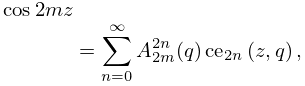
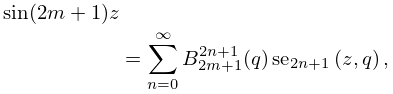
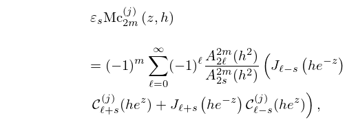
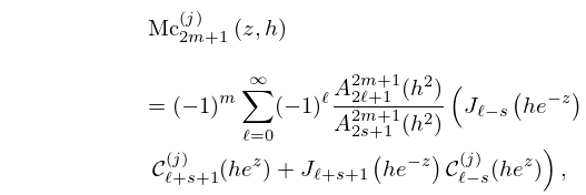
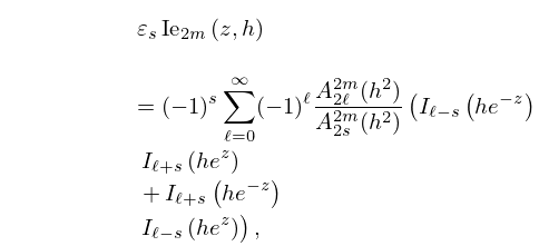
13: 28.11 Expansions in Series of Mathieu Functions

… ►

28.11.3 $$1=2\sum _{n=0}^{\mathrm{\infty }}{A}_0^{2n}(q){\mathrm{ce}}_{2n}(z,q),$$

ⓘ

Symbols:

${\mathrm{ce}}_n(z,q)$: Mathieu function, $q=h^2$: parameter, $n$: integer, $z$: complex variable and $A_m(q)$: Fourier coefficient

Permalink:

http://dlmf.nist.gov/28.11.E3

Encodings:

pMML, png, TeX

See also:

Annotations for §28.11, §28.11 and Ch.28

►

28.11.4 $$\cos 2mz=\sum _{n=0}^{\mathrm{\infty }}{A}_{2m}^{2n}(q){\mathrm{ce}}_{2n}(z,q),$$ $m\ne 0$,

ⓘ

Symbols:

${\mathrm{ce}}_n(z,q)$: Mathieu function, $\cos z$: cosine function, $m$: integer, $q=h^2$: parameter, $n$: integer, $z$: complex variable and $A_m(q)$: Fourier coefficient

Permalink:

http://dlmf.nist.gov/28.11.E4

Encodings:

pMML, png, TeX

See also:

Annotations for §28.11, §28.11 and Ch.28

►

28.11.5 $$\cos (2m+1)z=\sum _{n=0}^{\mathrm{\infty }}{A}_{2m+1}^{2n+1}(q){\mathrm{ce}}_{2n+1}(z,q),$$

ⓘ

Symbols:

${\mathrm{ce}}_n(z,q)$: Mathieu function, $\cos z$: cosine function, $m$: integer, $q=h^2$: parameter, $n$: integer, $z$: complex variable and $A_m(q)$: Fourier coefficient

Permalink:

http://dlmf.nist.gov/28.11.E5

Encodings:

pMML, png, TeX

See also:

Annotations for §28.11, §28.11 and Ch.28

►

28.11.6 $$\sin (2m+1)z=\sum _{n=0}^{\mathrm{\infty }}{B}_{2m+1}^{2n+1}(q){\mathrm{se}}_{2n+1}(z,q),$$

ⓘ

Symbols:

${\mathrm{se}}_n(z,q)$: Mathieu function, $\sin z$: sine function, $m$: integer, $q=h^2$: parameter, $n$: integer, $z$: complex variable and $B_m(q)$: Fourier coefficient

Permalink:

http://dlmf.nist.gov/28.11.E6

Encodings:

pMML, png, TeX

See also:

Annotations for §28.11, §28.11 and Ch.28

►

28.11.7 $$\sin (2m+2)z=\sum _{n=0}^{\mathrm{\infty }}{B}_{2m+2}^{2n+2}(q){\mathrm{se}}_{2n+2}(z,q).$$

ⓘ

Symbols:

${\mathrm{se}}_n(z,q)$: Mathieu function, $\sin z$: sine function, $m$: integer, $q=h^2$: parameter, $n$: integer, $z$: complex variable and $B_m(q)$: Fourier coefficient

Permalink:

http://dlmf.nist.gov/28.11.E7

Encodings:

pMML, png, TeX

See also:

Annotations for §28.11, §28.11 and Ch.28

14: 6.16 Mathematical Applications

… ►Consider the Fourier series … ►Compare Figure 6.16.1. … ►It occurs with Fourier-series expansions of all piecewise continuous functions. … …

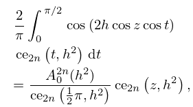
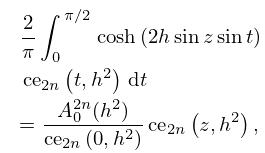
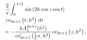
15: 28.35 Tables

§28.35 Tables

… ►

Ince (1932) includes eigenvalues $a_n$, $b_n$, and Fourier coefficients for $n=0$ or $1(1)6$, $q=0(1)10(2)20(4)40$; 7D. Also ${\mathrm{ce}}_n(x,q)$, ${\mathrm{se}}_n(x,q)$ for $q=0(1)10$, $x=1(1)90$, corresponding to the eigenvalues in the tables; 5D. Notation: $a_n={\mathrm{𝑏𝑒}}_n-2q$, $b_n={\mathrm{𝑏𝑜}}_n-2q$.

… ►

National Bureau of Standards (1967) includes the eigenvalues $a_n\left(q\right)$, $b_n\left(q\right)$ for $n=0(1)3$ with $q=0(.2)20(.5)37(1)100$, and $n=4(1)15$ with $q=0(2)100$; Fourier coefficients for ${\mathrm{ce}}_n(x,q)$ and ${\mathrm{se}}_n(x,q)$ for $n=0(1)15$, $n=1(1)15$, respectively, and various values of $q$ in the interval $[0,100]$; joining factors $g_{e,n}(\sqrt{q})$, $f_{e,n}(\sqrt{q})$ for $n=0(1)15$ with $q=0(.5\text{ to }10)100$ (but in a different notation). Also, eigenvalues for large values of $q$. Precision is generally 8D.

►

Stratton et al. (1941) includes $b_n$, $b_n^{\prime }$, and the corresponding Fourier coefficients for ${\mathrm{Se}}_n(c,x)$ and ${\mathrm{So}}_n(c,x)$ for $n=0$ or $1(1)4$, $c=0(.1\text{or}.2)4.5$. Precision is mostly 5S. Notation: $c=2\sqrt{q}$, $b_n=a_n+2q$, $b_n^{\prime }=b_n+2q$, and for ${\mathrm{Se}}_n(c,x)$, ${\mathrm{So}}_n(c,x)$ see §28.1.

… ►

Blanch and Clemm (1969) includes eigenvalues $a_n\left(q\right)$, $b_n\left(q\right)$ for $q=\rho {\mathrm{e}}^{\mathrm{i}\varphi }$, $\rho =0(.5)25$, $\varphi =5^{\circ }(5^{\circ }){90}^{\circ }$, $n=0(1)15$; 4D. Also $a_n\left(q\right)$ and $b_n\left(q\right)$ for $q=\mathrm{i}\rho$, $\rho =0(.5)100$, $n=0(2)14$ and $n=2(2)16$, respectively; 8D. Double points for $n=0(1)15$; 8D. Graphs are included.

…

16: 21.10 Methods of Computation

… ►In addition to evaluating the Fourier series, the main problem here is to compute a Riemann matrix originating from a Riemann surface. …

17: 27.10 Periodic Number-Theoretic Functions

… ►Every function periodic (mod $k$) can be expressed as a finite Fourier series of the form … ►is a periodic function of $n(modk)$ and has the finite Fourier-series expansion … ►The finite Fourier expansion of a primitive Dirichlet character $\chi (modk)$ has the form …

18: 24.8 Series Expansions

… ►

§24.8(i) Fourier Series

… ►If $n=1,2,\mathrm{\dots }$ and $0\le x\le 1$, then …

19: 28.24 Expansions in Series of Cross-Products of Bessel Functions or Modified Bessel Functions

… ►

28.24.2 $${\epsilon }_s{\mathrm{Mc}}_{2m}^{(j)}(z,h)={(-1)}^m\sum _{\mathrm{\ell }=0}^{\mathrm{\infty }}{(-1)}^{\mathrm{\ell }}\frac{A_{2\mathrm{\ell }}^{2m}(h^2)}{A_{2s}^{2m}(h^2)}\left(J_{\mathrm{\ell }-s}\left(h{\mathrm{e}}^{-z}\right){𝒞}_{\mathrm{\ell }+s}^{(j)}(h{\mathrm{e}}^z)+J_{\mathrm{\ell }+s}\left(h{\mathrm{e}}^{-z}\right){𝒞}_{\mathrm{\ell }-s}^{(j)}(h{\mathrm{e}}^z)\right),$$

ⓘ

Symbols:

$J_{\nu }\left(z\right)$: Bessel function of the first kind, $\mathrm{e}$: base of natural logarithm, ${\mathrm{Mc}}_n^{(j)}(z,h)$: radial Mathieu function, $m$: integer, $h$: parameter, $j$: integer, $z$: complex variable, ${𝒞}_{\mu }^{(j)}$: cylinder functions, ${\epsilon }_s$: constants and $A_m(q)$: Fourier coefficient

A&S Ref:

20.6.7

Permalink:

http://dlmf.nist.gov/28.24.E2

Encodings:

pMML, png, TeX

See also:

Annotations for §28.24 and Ch.28

►

28.24.3 $${\mathrm{Mc}}_{2m+1}^{(j)}(z,h)={(-1)}^m\sum _{\mathrm{\ell }=0}^{\mathrm{\infty }}{(-1)}^{\mathrm{\ell }}\frac{A_{2\mathrm{\ell }+1}^{2m+1}(h^2)}{A_{2s+1}^{2m+1}(h^2)}\left(J_{\mathrm{\ell }-s}\left(h{\mathrm{e}}^{-z}\right){𝒞}_{\mathrm{\ell }+s+1}^{(j)}(h{\mathrm{e}}^z)+J_{\mathrm{\ell }+s+1}\left(h{\mathrm{e}}^{-z}\right){𝒞}_{\mathrm{\ell }-s}^{(j)}(h{\mathrm{e}}^z)\right),$$

ⓘ

Symbols:

$J_{\nu }\left(z\right)$: Bessel function of the first kind, $\mathrm{e}$: base of natural logarithm, ${\mathrm{Mc}}_n^{(j)}(z,h)$: radial Mathieu function, $m$: integer, $h$: parameter, $j$: integer, $z$: complex variable, ${𝒞}_{\mu }^{(j)}$: cylinder functions and $A_m(q)$: Fourier coefficient

A&S Ref:

20.6.8

Permalink:

http://dlmf.nist.gov/28.24.E3

Encodings:

pMML, png, TeX

See also:

Annotations for §28.24 and Ch.28

►

28.24.4 $${\mathrm{Ms}}_{2m+1}^{(j)}(z,h)={(-1)}^m\sum _{\mathrm{\ell }=0}^{\mathrm{\infty }}{(-1)}^{\mathrm{\ell }}\frac{B_{2\mathrm{\ell }+1}^{2m+1}(h^2)}{B_{2s+1}^{2m+1}(h^2)}\left(J_{\mathrm{\ell }-s}\left(h{\mathrm{e}}^{-z}\right){𝒞}_{\mathrm{\ell }+s+1}^{(j)}(h{\mathrm{e}}^z)-J_{\mathrm{\ell }+s+1}\left(h{\mathrm{e}}^{-z}\right){𝒞}_{\mathrm{\ell }-s}^{(j)}(h{\mathrm{e}}^z)\right),$$

ⓘ

Symbols:

$J_{\nu }\left(z\right)$: Bessel function of the first kind, $\mathrm{e}$: base of natural logarithm, ${\mathrm{Ms}}_n^{(j)}(z,h)$: radial Mathieu function, $m$: integer, $h$: parameter, $j$: integer, $z$: complex variable, ${𝒞}_{\mu }^{(j)}$: cylinder functions and $B_m(q)$: Fourier coefficient

A&S Ref:

20.6.9

Permalink:

http://dlmf.nist.gov/28.24.E4

Encodings:

pMML, png, TeX

See also:

Annotations for §28.24 and Ch.28

►

28.24.5 $${\mathrm{Ms}}_{2m+2}^{(j)}(z,h)={(-1)}^m\sum _{\mathrm{\ell }=0}^{\mathrm{\infty }}{(-1)}^{\mathrm{\ell }}\frac{B_{2\mathrm{\ell }+2}^{2m+2}(h^2)}{B_{2s+2}^{2m+2}(h^2)}\left(J_{\mathrm{\ell }-s}\left(h{\mathrm{e}}^{-z}\right){𝒞}_{\mathrm{\ell }+s+2}^{(j)}(h{\mathrm{e}}^z)-J_{\mathrm{\ell }+s+2}\left(h{\mathrm{e}}^{-z}\right){𝒞}_{\mathrm{\ell }-s}^{(j)}(h{\mathrm{e}}^z)\right),$$

ⓘ

Symbols:

$J_{\nu }\left(z\right)$: Bessel function of the first kind, $\mathrm{e}$: base of natural logarithm, ${\mathrm{Ms}}_n^{(j)}(z,h)$: radial Mathieu function, $m$: integer, $h$: parameter, $j$: integer, $z$: complex variable, ${𝒞}_{\mu }^{(j)}$: cylinder functions and $B_m(q)$: Fourier coefficient

A&S Ref:

20.6.10

Permalink:

http://dlmf.nist.gov/28.24.E5

Encodings:

pMML, png, TeX

See also:

Annotations for §28.24 and Ch.28

… ►

28.24.6 $${\epsilon }_s{\mathrm{Ie}}_{2m}(z,h)={(-1)}^s\sum _{\mathrm{\ell }=0}^{\mathrm{\infty }}{(-1)}^{\mathrm{\ell }}\frac{A_{2\mathrm{\ell }}^{2m}(h^2)}{A_{2s}^{2m}(h^2)}\left(I_{\mathrm{\ell }-s}\left(h{\mathrm{e}}^{-z}\right)I_{\mathrm{\ell }+s}\left(h{\mathrm{e}}^z\right)+I_{\mathrm{\ell }+s}\left(h{\mathrm{e}}^{-z}\right)I_{\mathrm{\ell }-s}\left(h{\mathrm{e}}^z\right)\right),$$

ⓘ

Symbols:

$\mathrm{e}$: base of natural logarithm, $I_{\nu }\left(z\right)$: modified Bessel function of the first kind, ${\mathrm{Ie}}_n(z,h)$: modified Mathieu function, $m$: integer, $h$: parameter, $z$: complex variable, ${\epsilon }_s$: constants and $A_m(q)$: Fourier coefficient

A&S Ref:

20.8.8

Permalink:

http://dlmf.nist.gov/28.24.E6

Encodings:

pMML, png, TeX

See also:

Annotations for §28.24 and Ch.28

…

20: 28.10 Integral Equations

… ►With the notation of §28.4 for Fourier coefficients, ►

28.10.1 $$\frac{2}{\pi }{\int }_0^{\pi /2}\cos \left(2h\cos z\cos t\right){\mathrm{ce}}_{2n}(t,h^2)dt=\frac{A_0^{2n}(h^2)}{{\mathrm{ce}}_{2n}(\frac{1}{2}\pi ,h^2)}{\mathrm{ce}}_{2n}(z,h^2),$$

ⓘ

Symbols:

${\mathrm{ce}}_n(z,q)$: Mathieu function, $\pi$: the ratio of the circumference of a circle to its diameter, $\cos z$: cosine function, $dx$: differential of $x$ , $\int$: integral, $h$: parameter, $n$: integer, $z$: complex variable and $A_m(q)$: Fourier coefficient

A&S Ref:

20.7.20 (in different form)

Permalink:

http://dlmf.nist.gov/28.10.E1

Encodings:

pMML, png, TeX

See also:

Annotations for §28.10(i), §28.10 and Ch.28

►

28.10.2 $$\frac{2}{\pi }{\int }_0^{\pi /2}\cosh \left(2h\sin z\sin t\right){\mathrm{ce}}_{2n}(t,h^2)dt=\frac{A_0^{2n}(h^2)}{{\mathrm{ce}}_{2n}(0,h^2)}{\mathrm{ce}}_{2n}(z,h^2),$$

ⓘ

Symbols:

${\mathrm{ce}}_n(z,q)$: Mathieu function, $\pi$: the ratio of the circumference of a circle to its diameter, $dx$: differential of $x$ , $\cosh z$: hyperbolic cosine function, $\int$: integral, $\sin z$: sine function, $h$: parameter, $n$: integer, $z$: complex variable and $A_m(q)$: Fourier coefficient

A&S Ref:

20.7.21 (in different form)

Permalink:

http://dlmf.nist.gov/28.10.E2

Encodings:

pMML, png, TeX

See also:

Annotations for §28.10(i), §28.10 and Ch.28

►

28.10.3 $$\frac{2}{\pi }{\int }_0^{\pi /2}\sin \left(2h\cos z\cos t\right){\mathrm{ce}}_{2n+1}(t,h^2)dt=-\frac{h{A}_1^{2n+1}(h^2)}{{\mathrm{ce}}_{2n+1}^{\prime }(\frac{1}{2}\pi ,h^2)}{\mathrm{ce}}_{2n+1}(z,h^2),$$

ⓘ

Symbols:

${\mathrm{ce}}_n(z,q)$: Mathieu function, $\pi$: the ratio of the circumference of a circle to its diameter, $\cos z$: cosine function, $dx$: differential of $x$ , $\int$: integral, $\sin z$: sine function, $h$: parameter, $n$: integer, $z$: complex variable and $A_m(q)$: Fourier coefficient

A&S Ref:

20.7.20 (in different form)

Permalink:

http://dlmf.nist.gov/28.10.E3

Encodings:

pMML, png, TeX

See also:

Annotations for §28.10(i), §28.10 and Ch.28

… ►

28.10.5 $$\frac{2}{\pi }{\int }_0^{\pi /2}\sinh \left(2h\sin z\sin t\right){\mathrm{se}}_{2n+1}(t,h^2)dt=\frac{h{B}_1^{2n+1}(h^2)}{{\mathrm{se}}_{2n+1}^{\prime }(0,h^2)}{\mathrm{se}}_{2n+1}(z,h^2),$$

ⓘ

Symbols:

${\mathrm{se}}_n(z,q)$: Mathieu function, $\pi$: the ratio of the circumference of a circle to its diameter, $dx$: differential of $x$ , $\sinh z$: hyperbolic sine function, $\int$: integral, $\sin z$: sine function, $h$: parameter, $n$: integer, $z$: complex variable and $B_m(q)$: Fourier coefficient

A&S Ref:

20.7.23 (in different form)

Permalink:

http://dlmf.nist.gov/28.10.E5

Encodings:

pMML, png, TeX

See also:

Annotations for §28.10(i), §28.10 and Ch.28

…