F-homotopic transformations

SearchAdvancedHelp

(0.002 seconds)

21—30 of 169 matching pages

21: 6.14 Integrals

… ►

§6.14(i) Laplace Transforms

…

22: 23.18 Modular Transformations

§23.18 Modular Transformations

… ►

23.18.3 $$\lambda \left(𝒜\tau \right)=\lambda \left(\tau \right),$$

ⓘ

Symbols:

$\lambda \left(\tau \right)$: elliptic modular function, $\tau$: complex variable and $𝒜$: bilinear transformation

Permalink:

http://dlmf.nist.gov/23.18.E3

Encodings:

pMML, png, TeX

See also:

Annotations for §23.18, §23.18 and Ch.23

… ►

23.18.4 $$J\left(𝒜\tau \right)=J\left(\tau \right).$$

ⓘ

Symbols:

$J\left(\tau \right)$: Klein’s complete invariant, $\tau$: complex variable and $𝒜$: bilinear transformation

Referenced by:

§23.18

Permalink:

http://dlmf.nist.gov/23.18.E4

Encodings:

pMML, png, TeX

See also:

Annotations for §23.18, §23.18 and Ch.23

… ►

23.18.5 $$\eta \left(𝒜\tau \right)=\epsilon (𝒜){\left(-\mathrm{i}(c\tau +d)\right)}^{1/2}\eta \left(\tau \right),$$

ⓘ

Symbols:

$\eta \left(\tau \right)$: Dedekind’s eta function (or Dedekind modular function), $\mathrm{i}$: imaginary unit, $\tau$: complex variable, $𝒜$: bilinear transformation, $c$: integer, $d$: integer and $\epsilon (𝒜)$: function

Permalink:

http://dlmf.nist.gov/23.18.E5

Encodings:

pMML, png, TeX

See also:

Annotations for §23.18, §23.18 and Ch.23

… ►

23.18.6 $$\epsilon (𝒜)=\exp \left(\pi \mathrm{i}\left(\frac{a+d}{12c}+s(-d,c)\right)\right),$$

ⓘ

Symbols:

$\pi$: the ratio of the circumference of a circle to its diameter, $\exp z$: exponential function, $\mathrm{i}$: imaginary unit, $𝒜$: bilinear transformation, $a$: integer, $c$: integer, $d$: integer and $\epsilon (𝒜)$: function

Permalink:

http://dlmf.nist.gov/23.18.E6

Encodings:

pMML, png, TeX

See also:

Annotations for §23.18, §23.18 and Ch.23

…

23: Mark J. Ablowitz

… ►for appropriate data they can be linearized by the Inverse Scattering Transform (IST) and they possess solitons as special solutions. …Some of the relationships between IST and Painlevé equations are discussed in two books: Solitons and the Inverse Scattering Transform and Solitons, Nonlinear Evolution Equations and Inverse Scattering. …

24: 13.23 Integrals

… ►

§13.23(i) Laplace and Mellin Transforms

… ►

§13.23(ii) Fourier Transforms

… ►

§13.23(iii) Hankel Transforms

… ► ►

§13.23(iv) Integral Transforms in terms of Whittaker Functions

…

25: 22.17 Moduli Outside the Interval [0,1]

… ►

§22.17(ii) Complex Moduli

… ►In particular, the Landen transformations in §§22.7(i) and 22.7(ii) are valid for all complex values of $k$, irrespective of which values of $\sqrt{k}$ and $k^{\prime }=\sqrt{1-k^2}$ are chosen—as long as they are used consistently. …

26: 13.10 Integrals

… ►

§13.10(ii) Laplace Transforms

… ►

§13.10(iii) Mellin Transforms

… ►

§13.10(iv) Fourier Transforms

… ►

§13.10(v) Hankel Transforms

… ► …

27: 10.74 Methods of Computation

… ►

Hankel Transform

… ►

Spherical Bessel Transform

►The spherical Bessel transform is the Hankel transform (10.22.76) in the case when $\nu$ is half an odd positive integer. … ►

Kontorovich–Lebedev Transform

…

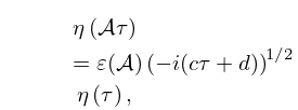
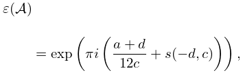
28: 21.5 Modular Transformations

§21.5 Modular Transformations

►

§21.5(i) Riemann Theta Functions

… ►Equation (21.5.4) is the modular transformation property for Riemann theta functions. … ►

§21.5(ii) Riemann Theta Functions with Characteristics

… ►For explicit results in the case $g=1$, see §20.7(viii).

29: 15.19 Methods of Computation

… ►For $z\in ℝ$ it is always possible to apply one of the linear transformations in §15.8(i) in such a way that the hypergeometric function is expressed in terms of hypergeometric functions with an argument in the interval $[0,\frac{1}{2}]$. ►For $z\in ℂ$ it is possible to use the linear transformations in such a way that the new arguments lie within the unit circle, except when $z={\mathrm{e}}^{\pm \pi \mathrm{i}/3}$. This is because the linear transformations map the pair $\{{\mathrm{e}}^{\pi \mathrm{i}/3},{\mathrm{e}}^{-\pi \mathrm{i}/3}\}$ onto itself. … ►When $\mathrm{\Re }z>\frac{1}{2}$ it is better to begin with one of the linear transformations (15.8.4), (15.8.7), or (15.8.8). … …

30: Bibliography W

… ►

The cubic transformation of the hypergeometric function. Quart. J. Pure and Applied Math. 41, pp. 70–79.

ⓘ

External Links:

ZentralBlatt

Referenced by:

§15.8(v), §15.8(v).

Encodings:

BibTeX

… ►

Some transformations of generalized hypergeometric series. Proc. London Math. Soc. (2) 26 (2), pp. 257–272.

ⓘ

External Links:

Document, ZentralBlatt

Referenced by:

§16.6.

Encodings:

BibTeX

… ►

The Airy transform. Amer. Math. Monthly 86 (4), pp. 271–277.

ⓘ

External Links:

ISSN 0002-9890, FullText, Document, MathReview (A. G. Ramm), ZentralBlatt

Referenced by:

(9.10.13), §9.10(ix), §9.10(v).

Encodings:

BibTeX

►

The Laplace Transform. Princeton Mathematical Series, v. 6, Princeton University Press, Princeton, NJ.

ⓘ

External Links:

FullText, MathReview (J. D. Tamarkin), ZentralBlatt

Referenced by:

§1.14(vi), §1.15(viii).

Encodings:

BibTeX

… ►

A class of integral transforms. Proc. Edinburgh Math. Soc. (2) 14, pp. 33–40.

ⓘ

External Links:

Document, MathReview (B. R. Bhonsle), ZentralBlatt

Referenced by:

§13.23(iv).

Encodings:

BibTeX

…