Euler%E2%80%93Maclaurin
(0.002 seconds)
1—10 of 413 matching pages
1: 24.1 Special Notation
…
►
Euler Numbers and Polynomials
… ►Its coefficients were first studied in Euler (1755); they were called Euler numbers by Raabe in 1851. The notations , , as defined in §24.2(ii), were used in Lucas (1891) and Nörlund (1924). …2: Bibliography H
…
►
The Laplace transform for expressions that contain a probability function.
Bul. Akad. Štiince RSS Moldoven. 1973 (2), pp. 78–80, 93 (Russian).
…
►
Note on Dr. Vacca’s series for
.
Quart. J. Math. 43, pp. 215–216.
…
►
An Euler-Maclaurin-type formula involving conjugate Bernoulli polynomials and an application to
.
Commun. Appl. Anal. 1 (1), pp. 15–32.
►
A Boole-type Formula involving Conjugate Euler Polynomials.
In Charlemagne and his Heritage. 1200 Years of Civilization and
Science in Europe, Vol. 2 (Aachen, 1995), P.L. Butzer, H. Th. Jongen, and W. Oberschelp (Eds.),
pp. 361–375.
…
►
Roots of the Euler polynomials.
Pacific J. Math. 64 (1), pp. 181–191.
…
3: 27.2 Functions
…
►This is the number of positive integers that are relatively prime to ; is Euler’s totient.
►If , then the Euler–Fermat theorem states that
…The numbers are relatively prime to and distinct (mod ).
…Note that .
…
►Table 27.2.2 tabulates the Euler totient function , the divisor function (), and the sum of the divisors (), for .
…
4: 24.17 Mathematical Applications
§24.17 Mathematical Applications
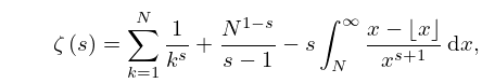
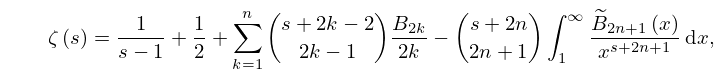
… ►Euler–Maclaurin Summation Formula
… ►Euler Splines
… ►are called Euler splines of degree . … ►5: 5.7 Series Expansions
…
►
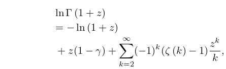
§5.7(i) Maclaurin and Taylor Series
… ►where , , and … ►
5.7.3
.
…
►For 20D numerical values of the coefficients of the Maclaurin series for see Luke (1969b, p. 299).
…
►
5.7.6
…
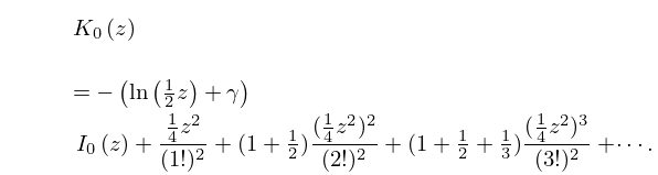
6: 10.31 Power Series
7: 31.3 Basic Solutions
…
►
denotes the solution of (31.2.1) that corresponds to the exponent at and assumes the value there.
If the other exponent is not a positive integer, that is, if , then from §2.7(i) it follows that exists, is analytic in the disk , and has the Maclaurin expansion
…
►Similarly, if , then the solution of (31.2.1) that corresponds to the exponent at is
…
►When , linearly independent solutions can be constructed as in §2.7(i).
…
►For example, is equal to
…
8: 24.18 Physical Applications
§24.18 Physical Applications
►Bernoulli polynomials appear in statistical physics (Ordóñez and Driebe (1996)), in discussions of Casimir forces (Li et al. (1991)), and in a study of quark-gluon plasma (Meisinger et al. (2002)). ►Euler polynomials also appear in statistical physics as well as in semi-classical approximations to quantum probability distributions (Ballentine and McRae (1998)).9: 12.12 Integrals
…
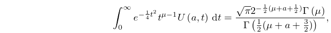
►
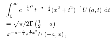
12.12.1
,
►
12.12.2
,
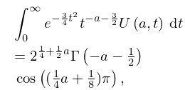
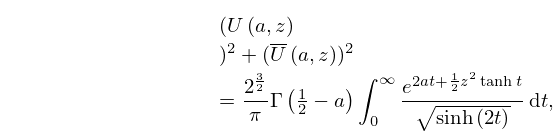
►
12.12.3
.
…
►
12.12.4
.
…
►For compendia of integrals see Erdélyi et al. (1953b, v. 2, pp. 121–122), Erdélyi et al. (1954a, b, v. 1, pp. 60–61, 115, 210–211, and 336;
v. 2, pp. 76–80, 115, 151, 171, and 395–398), Gradshteyn and Ryzhik (2000, §7.7), Magnus et al. (1966, pp. 330–331), Marichev (1983, pp. 190–191), Oberhettinger (1974, pp. 144–145), Oberhettinger (1990, pp. 106–108 and 192), Oberhettinger and Badii (1973, pp. 181–185), Prudnikov et al. (1986b, pp. 36–37, 155–168, 243–246, 289–290, 327–328, 419–420, and 619), Prudnikov et al. (1992a, §3.11), and Prudnikov et al. (1992b, §3.11).
…
