Euler%20integral

SearchAdvancedHelp

(0.004 seconds)

1—10 of 25 matching pages

1: Software Index

… ► ►►►►►►►

	Open Source													With Book						Commercial
…
11.16(iii) Integrals of …														✓					✓		✓	✓	a
…
11.16(vi) Integrals of …														✓							✓	✓	a
…
19 Elliptic Integrals
…
20 Theta Functions
…
24 Bernoulli and Euler Polynomials
…

…

2: 25.5 Integral Representations

§25.5 Integral Representations

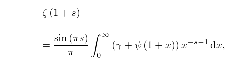
… ►In (25.5.15)–(25.5.19), , $\psi \left(x\right)$ is the digamma function, and $\gamma$ is Euler’s constant (§5.2). … ►

25.5.17 $$\zeta \left(1+s\right)=\frac{\sin \left(\pi s\right)}{\pi }{\int }_0^{\mathrm{\infty }}\left(\gamma +\psi \left(1+x\right)\right)x^{-s-1}dx,$$

ⓘ

Symbols:

$\gamma$: Euler’s constant, $\zeta \left(s\right)$: Riemann zeta function, $\pi$: the ratio of the circumference of a circle to its diameter, $dx$: differential of $x$ , $\psi \left(z\right)$: psi (or digamma) function, $\int$: integral, $\sin z$: sine function, $x$: real variable and $s$: complex variable

Keywords:

improper integral, integral representation

Source:

de Bruijn (1937, (22), p. 177)

Permalink:

http://dlmf.nist.gov/25.5.E17

Encodings:

pMML, png, TeX

See also:

Annotations for §25.5(ii), §25.5 and Ch.25

… ►

25.5.19 $$\zeta \left(m+s\right)={(-1)}^{m-1}\frac{\mathrm{\Gamma }\left(s\right)\sin \left(\pi s\right)}{\pi \mathrm{\Gamma }\left(m+s\right)}{\int }_0^{\mathrm{\infty }}{\psi }^{(m)}\left(1+x\right)x^{-s}dx,$$ $m=1,2,3,\mathrm{\dots }$.

ⓘ

Symbols:

$\mathrm{\Gamma }\left(z\right)$: gamma function, $\zeta \left(s\right)$: Riemann zeta function, $\pi$: the ratio of the circumference of a circle to its diameter, $dx$: differential of $x$ , $\psi \left(z\right)$: psi (or digamma) function, $\int$: integral, $\sin z$: sine function, $m$: nonnegative integer, $x$: real variable and $s$: complex variable

Keywords:

improper integral, integral representation

Source:

de Bruijn (1937, p. 178)

Referenced by:

§25.5(ii)

Permalink:

http://dlmf.nist.gov/25.5.E19

Encodings:

pMML, png, TeX

See also:

Annotations for §25.5(ii), §25.5 and Ch.25

►

§25.5(iii) Contour Integrals

…

3: Bibliography L

… ►

Algorithm 917: complex double-precision evaluation of the Wright $\omega$ function. ACM Trans. Math. Software 38 (3), pp. Art. 20, 17.

ⓘ

External Links:

ISSN 0098-3500, Document, FullText, MathReview Entry, ZentralBlatt

Referenced by:

§4.13, 2nd item, §4.48(iv).

Encodings:

BibTeX

… ►

An asymptotic estimate for the Bernoulli and Euler numbers. Canad. Math. Bull. 20 (1), pp. 109–111.

ⓘ

External Links:

MathReview (D. H. Lehmer), ZentralBlatt

Referenced by:

§24.11.

Encodings:

BibTeX

… ►

Hermite polynomials in asymptotic representations of generalized Bernoulli, Euler, Bessel, and Buchholz polynomials. J. Math. Anal. Appl. 239 (2), pp. 457–477.

ⓘ

External Links:

ISSN 0022-247X, Document, MathReview (A. G. Law), ZentralBlatt

Referenced by:

§18.34(iii), §24.11, §24.16(i), §24.16(i).

Encodings:

BibTeX

►

Uniform approximations of Bernoulli and Euler polynomials in terms of hyperbolic functions. Stud. Appl. Math. 103 (3), pp. 241–258.

ⓘ

External Links:

ISSN 0022-2526, Document, Link, MathReview, ZentralBlatt

Referenced by:

§24.11, §24.11.

Encodings:

BibTeX

… ►

Large degree asymptotics of generalized Bernoulli and Euler polynomials. J. Math. Anal. Appl. 363 (1), pp. 197–208.

ⓘ

External Links:

ISSN 0022-247X, Document, Link, MathReview (Richard B. Paris), ZentralBlatt

Referenced by:

§24.16(i), §24.16(i).

Encodings:

BibTeX

…

4: 20.10 Integrals

§20.10 Integrals

… ►

20.10.1 $${\int }_0^{\mathrm{\infty }}{x}^{s-1}{\theta }_2\left(0\right|\mathrm{i}{x}^2)dx=2^s(1-2^{-s}){\pi }^{-s/2}\mathrm{\Gamma }\left(\frac{1}{2}s\right)\zeta \left(s\right),$$ $\mathrm{\Re }s>1$,

ⓘ

Symbols:

$\mathrm{\Gamma }\left(z\right)$: gamma function, ${\theta }_j\left(z\right|\tau )$: theta function, $\zeta \left(s\right)$: Riemann zeta function, $\pi$: the ratio of the circumference of a circle to its diameter, $dx$: differential of $x$ , $\mathrm{i}$: imaginary unit, $\int$: integral and $\mathrm{\Re }$: real part

Keywords:

Mellin transform

Referenced by:

§20.10(i), Erratum (V1.1.5) for §20.10(i)

Permalink:

http://dlmf.nist.gov/20.10.E1

Encodings:

pMML, png, TeX

Modification (effective with 1.1.5):

Originally the constraint was $\mathrm{\Re }s>2$. This can be relaxed to $\mathrm{\Re }s>1$ because ${\theta }_2\left(0\right|\mathrm{i}{x}^2)=x^{-1}{\theta }_4\left(0\right|\mathrm{i}{x}^{-2})\sim x^{-1}$ as $x\to 0+$, which follows from (20.7.31) and (20.4.5).

See also:

Annotations for §20.10(i), §20.10 and Ch.20

►

20.10.2 $${\int }_0^{\mathrm{\infty }}{x}^{s-1}({\theta }_3\left(0\right|\mathrm{i}{x}^2)-1)dx={\pi }^{-s/2}\mathrm{\Gamma }\left(\frac{1}{2}s\right)\zeta \left(s\right),$$ $\mathrm{\Re }s>1$,

ⓘ

Symbols:

$\mathrm{\Gamma }\left(z\right)$: gamma function, ${\theta }_j\left(z\right|\tau )$: theta function, $\zeta \left(s\right)$: Riemann zeta function, $\pi$: the ratio of the circumference of a circle to its diameter, $dx$: differential of $x$ , $\mathrm{i}$: imaginary unit, $\int$: integral and $\mathrm{\Re }$: real part

Keywords:

Mellin transform

Referenced by:

§20.10(i), Erratum (V1.1.5) for §20.10(i)

Permalink:

http://dlmf.nist.gov/20.10.E2

Encodings:

pMML, png, TeX

Modification (effective with 1.1.5):

Originally the constraint was $\mathrm{\Re }s>2$. This can be relaxed to $\mathrm{\Re }s>1$ because ${\theta }_3\left(0\right|\mathrm{i}{x}^2)=x^{-1}{\theta }_3\left(0\right|\mathrm{i}{x}^{-2})\sim x^{-1}$ as $x\to 0+$, which follows from (20.7.32) and (20.4.4).

See also:

Annotations for §20.10(i), §20.10 and Ch.20

►

20.10.3 $${\int }_0^{\mathrm{\infty }}{x}^{s-1}(1-{\theta }_4\left(0\right|\mathrm{i}{x}^2))dx=(1-2^{1-s}){\pi }^{-s/2}\mathrm{\Gamma }\left(\frac{1}{2}s\right)\zeta \left(s\right),$$ $\mathrm{\Re }s>0$.

ⓘ

Symbols:

$\mathrm{\Gamma }\left(z\right)$: gamma function, ${\theta }_j\left(z\right|\tau )$: theta function, $\zeta \left(s\right)$: Riemann zeta function, $\pi$: the ratio of the circumference of a circle to its diameter, $dx$: differential of $x$ , $\mathrm{i}$: imaginary unit, $\int$: integral and $\mathrm{\Re }$: real part

Keywords:

Mellin transform

Referenced by:

§20.10(i), Erratum (V1.1.5) for §20.10(i)

Permalink:

http://dlmf.nist.gov/20.10.E3

Encodings:

pMML, png, TeX

Modification (effective with 1.1.5):

Originally the constraint was $\mathrm{\Re }s>2$. This can be relaxed to $\mathrm{\Re }s>0$ because $1-{\theta }_4\left(0\right|\mathrm{i}{x}^2)=1-x^{-1}{\theta }_2\left(0\right|\mathrm{i}{x}^{-2})\sim 1$ as $x\to 0+$, which follows from (20.7.33) and (20.4.3).

See also:

Annotations for §20.10(i), §20.10 and Ch.20

… ►For further integrals of theta functions see Erdélyi et al. (1954a, pp. 61–62 and 339), Prudnikov et al. (1990, pp. 356–358), Prudnikov et al. (1992a, §3.41), and Gradshteyn and Ryzhik (2000, pp. 627–628).

5: 25.20 Approximations

… ►

Cody et al. (1971) gives rational approximations for $\zeta \left(s\right)$ in the form of quotients of polynomials or quotients of Chebyshev series. The ranges covered are $0.5\le s\le 5$, $5\le s\le 11$, $11\le s\le 25$, $25\le s\le 55$. Precision is varied, with a maximum of 20S.

… ►

Morris (1979) gives rational approximations for ${\mathrm{Li}}_2\left(x\right)$ (§25.12(i)) for $0.5\le x\le 1$. Precision is varied with a maximum of 24S.

►

Antia (1993) gives minimax rational approximations for $\mathrm{\Gamma }\left(s+1\right)F_s(x)$, where $F_s(x)$ is the Fermi–Dirac integral (25.12.14), for the intervals and , with $s=-\frac{1}{2},\frac{1}{2},\frac{3}{2},\frac{5}{2}$. For each $s$ there are three sets of approximations, with relative maximum errors ${10}^{-4},{10}^{-8},{10}^{-12}$.

6: 8.26 Tables

… ►

Khamis (1965) tabulates $P(a,x)$ for $a=0.05(.05)10(.1)20(.25)70$, $0.0001\le x\le 250$ to 10D.

… ►

§8.26(iv) Generalized Exponential Integral

►

Abramowitz and Stegun (1964, pp. 245–248) tabulates $E_n\left(x\right)$ for $n=2,3,4,10,20$, $x=0(.01)2$ to 7D; also $(x+n){\mathrm{e}}^x{E}_n\left(x\right)$ for $n=2,3,4,10,20$, $x^{-1}=0(.01)0.1(.05)0.5$ to 6S.

… ►

Pagurova (1961) tabulates $E_n\left(x\right)$ for $n=0(1)20$, $x=0(.01)2(.1)10$ to 4-9S; ${\mathrm{e}}^x{E}_n\left(x\right)$ for $n=2(1)10$, $x=10(.1)20$ to 7D; ${\mathrm{e}}^x{E}_p\left(x\right)$ for $p=0(.1)1$, $x=0.01(.01)7(.05)12(.1)20$ to 7S or 7D.

… ►

Zhang and Jin (1996, Table 19.1) tabulates $E_n\left(x\right)$ for $n=1,2,3,5,10,15,20$, $x=0(.1)1,1.5,2,3,5,10,20,30,50,100$ to 7D or 8S.

7: 25.11 Hurwitz Zeta Function

… ►

►►

Figure 25.11.1: Hurwitz zeta function $\zeta (x,a)$, $a$ = 0. …8, 1, $-20\le x\le 10$. … Magnify

… ►

§25.11(iii) Representations by the Euler–Maclaurin Formula

… ►

§25.11(vii) Integral Representations

… ►

§25.11(viii) Further Integral Representations

… ►

§25.11(ix) Integrals

…

8: 25.12 Polylogarithms

… ►The right-hand side is called Clausen’s integral. … ►

Integral Representation

… ►

§25.12(iii) Fermi–Dirac and Bose–Einstein Integrals

►The Fermi–Dirac and Bose–Einstein integrals are defined by … ►In terms of polylogarithms …

9: Bibliography

… ►

Exact linearization of a Painlevé transcendent. Phys. Rev. Lett. 38 (20), pp. 1103–1106.

ⓘ

External Links:

Document, MathReview (Mark Adler)

Referenced by:

§32.11(ii), §32.13(i), §32.13(ii), §32.13(iii), §32.5.

Encodings:

BibTeX

… ►

On the degrees of irreducible factors of higher order Bernoulli polynomials. Acta Arith. 62 (4), pp. 329–342.

ⓘ

External Links:

ISSN 0065-1036, Pdf, MathReview (L. Skula), ZentralBlatt

Referenced by:

§24.12(iii).

Encodings:

BibTeX

… ►

Application of the combined nonlinear-condensation transformation to problems in statistical analysis and theoretical physics. Comput. Phys. Comm. 150 (1), pp. 1–20.

ⓘ

Notes:

Includes algorithms for Lerch’s transcendent. C and Mathematica codes by Aksenov and Jentschura are available.

External Links:

Code, Document

Referenced by:

1st item.

Encodings:

BibTeX

… ►

Repeated integrals and derivatives of $K$ Bessel functions. SIAM J. Math. Anal. 20 (1), pp. 169–175.

ⓘ

External Links:

ISSN 0036-1410, Document, MathReview (A. Haimovici), ZentralBlatt

Referenced by:

§10.43(iii).

Encodings:

BibTeX

… ►

Numerical Tables for Angular Correlation Computations in $\alpha$-, $\beta$- and $\gamma$-Spectroscopy: $3j$-, $6j$-, $9j$-Symbols, F- and $\mathrm{\Gamma }$-Coefficients. Landolt-Börnstein Numerical Data and Functional Relationships in Science and Technology, Springer-Verlag.

ⓘ

External Links:

ISBN 978-3-540-04218-1

Referenced by:

§34.14.

Encodings:

BibTeX

…

10: 7.23 Tables

… ►

Abramowitz and Stegun (1964, Chapter 7) includes $\mathrm{erf}x$, $(2/\sqrt{\pi }){\mathrm{e}}^{-x^2}$, $x\in [0,2]$, 10D; $(2/\sqrt{\pi }){\mathrm{e}}^{-x^2}$, $x\in [2,10]$, 8S; $x{\mathrm{e}}^{x^2}\mathrm{erfc}x$, $x^{-2}\in [0,0.25]$, 7D; $2^n\mathrm{\Gamma }\left(\frac{1}{2}n+1\right){\mathrm{i}}^n\mathrm{erfc}\left(x\right)$, $n=1(1)6,10,11$, $x\in [0,5]$, 6S; $F\left(x\right)$, $x\in [0,2]$, 10D; $xF\left(x\right)$, $x^{-2}\in [0,0.25]$, 9D; $C\left(x\right)$, $S\left(x\right)$, $x\in [0,5]$, 7D; $\mathrm{f}\left(x\right)$, $\mathrm{g}\left(x\right)$, $x\in [0,1]$, $x^{-1}\in [0,1]$, 15D.

►

Abramowitz and Stegun (1964, Table 27.6) includes the Goodwin–Staton integral $G\left(x\right)$, $x=1(.1)3(.5)8$, 4D; also $G\left(x\right)+\ln x$, $x=0(.05)1$, 4D.

… ►

Zhang and Jin (1996, pp. 637, 639) includes $(2/\sqrt{\pi }){\mathrm{e}}^{-x^2}$, $\mathrm{erf}x$, $x=0(.02)1(.04)3$, 8D; $C\left(x\right)$, $S\left(x\right)$, $x=0(.2)10(2)100(100)500$, 8D.

… ►

Zhang and Jin (1996, pp. 638, 640–641) includes the real and imaginary parts of $\mathrm{erf}z$, $x\in [0,5]$, $y=0.5(.5)3$, 7D and 8D, respectively; the real and imaginary parts of ${\int }_x^{\mathrm{\infty }}{\mathrm{e}}^{\pm \mathrm{i}{t}^2}dt$, $(1/\sqrt{\pi }){\mathrm{e}}^{\mp \mathrm{i}(x^2+(\pi /4))}{\int }_x^{\mathrm{\infty }}{\mathrm{e}}^{\pm \mathrm{i}{t}^2}dt$, $x=0(.5)20(1)25$, 8D, together with the corresponding modulus and phase to 8D and 6D (degrees), respectively.

… ►

Zhang and Jin (1996, p. 642) includes the first 10 zeros of $\mathrm{erf}z$, 9D; the first 25 distinct zeros of $C\left(z\right)$ and $S\left(z\right)$, 8S.