Dougall%20expansion

SearchAdvancedHelp

(0.002 seconds)

1—10 of 343 matching pages

1: 16.4 Argument Unity

… ►

Rogers–Dougall Very Well-Poised Sum

… ►

Dougall’s Very Well-Poised Sum

… ►The function ${}_3{}^{}F_2^{}(a,b,c;d,e;1)$ is analytic in the parameters $a,b,c,d,e$ when its series expansion converges and the bottom parameters are not negative integers or zero. … ►This is Dougall’s bilateral sum; see Andrews et al. (1999, §2.8).

2: Bibliography D

… ►

Asymptotic Expansions: Their Derivation and Interpretation. Academic Press, London-New York.

ⓘ

External Links:

MathReview, ZentralBlatt

Referenced by:

(11.11.11), §11.6(i), §11.6(iii), §2.11(v), Ch.2, §8.1, Notations, Notations.

Encodings:

BibTeX

… ►

Complex zeros of cylinder functions. Math. Comp. 20 (94), pp. 215–222.

ⓘ

Notes:

For a numerical error in one of the zeros see Amos (1985).

External Links:

ISSN 0025-5718, FullText, MathReview, ZentralBlatt

Referenced by:

2nd item.

Encodings:

BibTeX

… ►

On Vandermonde’s theorem, and some more general expansions. Proc. Edinburgh Math. Soc. 25, pp. 114–132.

ⓘ

External Links:

ZentralBlatt

Referenced by:

§15.4(ii).

Encodings:

BibTeX

… ►

Uniform asymptotic expansions for Whittaker’s confluent hypergeometric functions. SIAM J. Math. Anal. 20 (3), pp. 744–760.

ⓘ

Notes:

(This reference has several typographical errors.)

External Links:

ISSN 0036-1410, Document, MathReview (F. W. J. Olver), ZentralBlatt

Referenced by:

§13.21(ii), §13.21(iii), §13.21(iv).

Encodings:

BibTeX

… ►

Uniform asymptotic expansions for Charlier polynomials. J. Approx. Theory 112 (1), pp. 93–133.

ⓘ

External Links:

ISSN 0021-9045, Document, MathReview (Eberhard Wagner), ZentralBlatt

Referenced by:

§18.24.

Encodings:

BibTeX

…

3: 14.18 Sums

… ►

§14.18(i) Expansion Theorem

►For expansions of arbitrary functions in series of Legendre polynomials see §18.18(i), and for expansions of arbitrary functions in series of associated Legendre functions see Schäfke (1961b). … ►

Dougall’s Expansion

…

4: 6.20 Approximations

… ►

Cody and Thacher (1968) provides minimax rational approximations for $E_1\left(x\right)$, with accuracies up to 20S.

►

Cody and Thacher (1969) provides minimax rational approximations for $\mathrm{Ei}\left(x\right)$, with accuracies up to 20S.

►

MacLeod (1996b) provides rational approximations for the sine and cosine integrals and for the auxiliary functions $\mathrm{f}$ and $\mathrm{g}$, with accuracies up to 20S.

►

§6.20(ii) Expansions in Chebyshev Series

… ►

§6.20(iii) Padé-Type and Rational Expansions

…

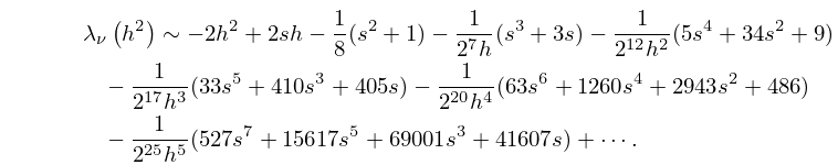
5: 28.16 Asymptotic Expansions for Large $q$

§28.16 Asymptotic Expansions for Large $q$

… ►

28.16.1 $${\lambda }_{\nu }\left(h^2\right)\sim -2h^2+2sh-\frac{1}{8}(s^2+1)-\frac{1}{2^{7}h}(s^3+3s)-\frac{1}{2^{12}{h}^2}(5s^4+34s^2+9)-\frac{1}{2^{17}{h}^3}(33s^5+410s^3+405s)-\frac{1}{2^{20}{h}^4}(63s^6+1260s^4+2943s^2+486)-\frac{1}{2^{25}{h}^5}(527s^7+15617s^5+69001s^3+41607s)+\mathrm{\cdots }.$$

ⓘ

Symbols:

${\lambda }_{\nu +2n}\left(q\right)$: eigenvalues of Mathieu equation, $\sim$: Poincaré asymptotic expansion, $h$: parameter and $\nu$: complex parameter

Permalink:

http://dlmf.nist.gov/28.16.E1

Encodings:

pMML, png, TeX

See also:

Annotations for §28.16 and Ch.28

…

6: 20 Theta Functions

Chapter 20 Theta Functions

…

7: 7.24 Approximations

… ►

Cody (1969) provides minimax rational approximations for $\mathrm{erf}x$ and $\mathrm{erfc}x$. The maximum relative precision is about 20S.

… ►

Cody et al. (1970) gives minimax rational approximations to Dawson’s integral $F\left(x\right)$ (maximum relative precision 20S–22S).

►

§7.24(ii) Expansions in Chebyshev Series

… ►

Schonfelder (1978) gives coefficients of Chebyshev expansions for $x^{-1}\mathrm{erf}x$ on $0\le x\le 2$, for $x{\mathrm{e}}^{x^2}\mathrm{erfc}x$ on $[2,\mathrm{\infty })$, and for ${\mathrm{e}}^{x^2}\mathrm{erfc}x$ on $[0,\mathrm{\infty })$ (30D).

… ►

§7.24(iii) Padé-Type Expansions

…

8: 25.20 Approximations

… ►

Cody et al. (1971) gives rational approximations for $\zeta \left(s\right)$ in the form of quotients of polynomials or quotients of Chebyshev series. The ranges covered are $0.5\le s\le 5$, $5\le s\le 11$, $11\le s\le 25$, $25\le s\le 55$. Precision is varied, with a maximum of 20S.

►

Piessens and Branders (1972) gives the coefficients of the Chebyshev-series expansions of $s\zeta \left(s+1\right)$ and $\zeta \left(s+k\right)$, $k=2,3,4,5,8$, for $0\le s\le 1$ (23D).

►

Luke (1969b, p. 306) gives coefficients in Chebyshev-series expansions that cover $\zeta \left(s\right)$ for $0\le s\le 1$ (15D), $\zeta \left(s+1\right)$ for $0\le s\le 1$ (20D), and $\ln \xi \left(\frac{1}{2}+\mathrm{i}x\right)$ (§25.4) for $-1\le x\le 1$ (20D). For errata see Piessens and Branders (1972).

…

9: 11.6 Asymptotic Expansions

§11.6 Asymptotic Expansions

… ►For re-expansions of the remainder terms in (11.6.1) and (11.6.2), see Dingle (1973, p. 445). … ►More fully, the series (11.2.1) and (11.2.2) can be regarded as generalized asymptotic expansions (§2.1(v)). … ►Here …

10: 10.75 Tables

… ►

Achenbach (1986) tabulates $J_0\left(x\right)$, $J_1\left(x\right)$, $Y_0\left(x\right)$, $Y_1\left(x\right)$, $x=0(.1)8$, 20D or 18–20S.

… ►

Olver (1960) tabulates $j_{n,m}$, $J_n^{\prime }\left(j_{n,m}\right)$, $j_{n,m}^{\prime }$, $J_n\left(j_{n,m}^{\prime }\right)$, $y_{n,m}$, $Y_n^{\prime }\left(y_{n,m}\right)$, $y_{n,m}^{\prime }$, $Y_n\left(y_{n,m}^{\prime }\right)$, $n=0(\frac{1}{2})20⁤\frac{1}{2}$, $m=1(1)50$, 8D. Also included are tables of the coefficients in the uniform asymptotic expansions of these zeros and associated values as $n\to \mathrm{\infty }$; see §10.21(viii), and more fully Olver (1954).

… ►

Bickley et al. (1952) tabulates $x^{-n}{I}_n\left(x\right)$ or ${\mathrm{e}}^{-x}{I}_n\left(x\right)$, $x^n{K}_n\left(x\right)$ or ${\mathrm{e}}^x{K}_n\left(x\right)$, $n=2(1)20$, $x=0$(.01 or .1) 10(.1) 20, 8S; $I_n\left(x\right)$, $K_n\left(x\right)$, $n=0(1)20$, $x=0$ or $0.1(.1)20$, 10S.

… ►

Kerimov and Skorokhodov (1984b) tabulates all zeros of the principal values of $K_n\left(z\right)$ and $K_n^{\prime }\left(z\right)$, for $n=2(1)20$, 9S.

… ►

Olver (1960) tabulates $a_{n,m}^{\prime }$, ${𝗃}_n\left(a_{n,m}^{\prime }\right)$, $b_{n,m}^{\prime }$, ${𝗒}_n\left(b_{n,m}^{\prime }\right)$, $n=1(1)20$, $m=1(1)50$, 8D. Also included are tables of the coefficients in the uniform asymptotic expansions of these zeros and associated values as $n\to \mathrm{\infty }$.

…