Coulomb%20phase%20shift

SearchAdvancedHelp

(0.003 seconds)

1—10 of 385 matching pages

1: 33.24 Tables

§33.24 Tables

►

Abramowitz and Stegun (1964, Chapter 14) tabulates $F_0(\eta ,\rho )$, $G_0(\eta ,\rho )$, $F_0^{\prime }(\eta ,\rho )$, and $G_0^{\prime }(\eta ,\rho )$ for $\eta =0.5(.5)20$ and $\rho =1(1)20$, 5S; $C_0\left(\eta \right)$ for $\eta =0(.05)3$, 6S.

…

2: 33.25 Approximations

§33.25 Approximations

►Cody and Hillstrom (1970) provides rational approximations of the phase shift ${\sigma }_0\left(\eta \right)=\mathrm{ph}\mathrm{\Gamma }\left(1+\mathrm{i}\eta \right)$ (see (33.2.10)) for the ranges $0\le \eta \le 2$, $2\le \eta \le 4$, and $4\le \eta \le \mathrm{\infty }$. …

3: 33.2 Definitions and Basic Properties

… ►

§33.2(i) Coulomb Wave Equation

… ► ${\sigma }_{\mathrm{\ell }}\left(\eta \right)$ is the Coulomb phase shift. … ►Also, ${\mathrm{e}}^{\mp \mathrm{i}{\sigma }_{\mathrm{\ell }}\left(\eta \right)}{H}_{\mathrm{\ell }}^{\pm }(\eta ,\rho )$ are analytic functions of $\eta$ when . ►

§33.2(iv) Wronskians and Cross-Product

…

4: 33.13 Complex Variable and Parameters

§33.13 Complex Variable and Parameters

►The functions $F_{\mathrm{\ell }}(\eta ,\rho )$, $G_{\mathrm{\ell }}(\eta ,\rho )$, and $H_{\mathrm{\ell }}^{\pm }(\eta ,\rho )$ may be extended to noninteger values of $\mathrm{\ell }$ by generalizing $(2\mathrm{\ell }+1)!=\mathrm{\Gamma }\left(2\mathrm{\ell }+2\right)$, and supplementing (33.6.5) by a formula derived from (33.2.8) with $U(a,b,z)$ expanded via (13.2.42). … ►The quantities $C_{\mathrm{\ell }}\left(\eta \right)$, ${\sigma }_{\mathrm{\ell }}\left(\eta \right)$, and $R_{\mathrm{\ell }}$, given by (33.2.6), (33.2.10), and (33.4.1), respectively, must be defined consistently so that ►

33.13.1 $$C_{\mathrm{\ell }}\left(\eta \right)=2^{\mathrm{\ell }}{\mathrm{e}}^{\mathrm{i}{\sigma }_{\mathrm{\ell }}\left(\eta \right)-(\pi \eta /2)}\mathrm{\Gamma }\left(\mathrm{\ell }+1-\mathrm{i}\eta \right)/\mathrm{\Gamma }\left(2\mathrm{\ell }+2\right),$$

ⓘ

Symbols:

$C_{\mathrm{\ell }}\left(\eta \right)$: normalizing constant for Coulomb radial functions, ${\sigma }_{\mathrm{\ell }}\left(\eta \right)$: Coulomb phase shift, $\mathrm{\Gamma }\left(z\right)$: gamma function, $\pi$: the ratio of the circumference of a circle to its diameter, $\mathrm{e}$: base of natural logarithm, $\mathrm{i}$: imaginary unit, $\mathrm{\ell }$: nonnegative integer and $\eta$: real parameter

Permalink:

http://dlmf.nist.gov/33.13.E1

Encodings:

pMML, png, TeX

See also:

Annotations for §33.13 and Ch.33

… ►

33.13.2 $$R_{\mathrm{\ell }}=(2\mathrm{\ell }+1)C_{\mathrm{\ell }}\left(\eta \right)/C_{\mathrm{\ell }-1}\left(\eta \right).$$

ⓘ

Symbols:

$C_{\mathrm{\ell }}\left(\eta \right)$: normalizing constant for Coulomb radial functions, $\mathrm{\ell }$: nonnegative integer, $\eta$: real parameter and $R_{\mathrm{\ell }}$: factor

Permalink:

http://dlmf.nist.gov/33.13.E2

Encodings:

pMML, png, TeX

See also:

Annotations for §33.13 and Ch.33

…

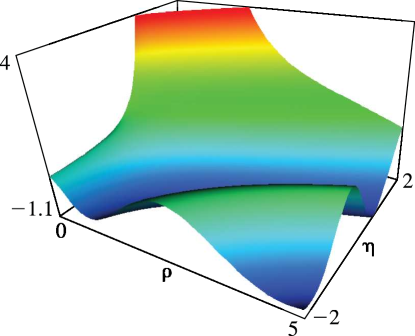
5: 33.3 Graphics

§33.3 Graphics

►

§33.3(i) Line Graphs of the Coulomb Radial Functions $F_{\mathrm{\ell }}(\eta ,\rho )$ and $G_{\mathrm{\ell }}(\eta ,\rho )$

… ►

►►

Figure 33.3.4: $F_{\mathrm{\ell }}(\eta ,\rho )$, $G_{\mathrm{\ell }}(\eta ,\rho )$ with $\mathrm{\ell }=0$, $\eta =10$. The turning point is at ${\rho }_{\mathrm{tp}}(10,0)=20$. Magnify

… ►

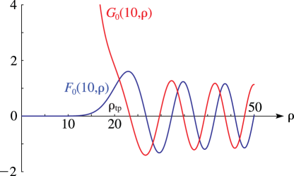§33.3(ii) Surfaces of the Coulomb Radial Functions $F_0(\eta ,\rho )$ and $G_0(\eta ,\rho )$

… ►

►

►

Figure 33.3.8: $G_0(\eta ,\rho )$, $-2\le \eta \le 2$, . Magnify 3D Help

6: 33.5 Limiting Forms for Small $\rho$, Small $|\eta |$, or Large $\mathrm{\ell }$

… ►

§33.5(i) Small $\rho$

… ►

§33.5(ii) $\eta =0$

… ►

§33.5(iii) Small $|\eta |$

►

33.5.7 $${\sigma }_0\left(\eta \right)\sim -\gamma \eta ,$$ $\eta \to 0$,

ⓘ

Symbols:

${\sigma }_{\mathrm{\ell }}\left(\eta \right)$: Coulomb phase shift, $\gamma$: Euler’s constant, $\sim$: asymptotic equality and $\eta$: real parameter

Permalink:

http://dlmf.nist.gov/33.5.E7

Encodings:

pMML, png, TeX

See also:

Annotations for §33.5(iii), §33.5 and Ch.33

… ►

§33.5(iv) Large $\mathrm{\ell }$

…

7: 33.23 Methods of Computation

§33.23 Methods of Computation

… ►The methods used for computing the Coulomb functions described below are similar to those in §13.29. … ►Combined with the Wronskians (33.2.12), the values of $F_{\mathrm{\ell }}$, $G_{\mathrm{\ell }}$, and their derivatives can be extracted. … ►

§33.23(vii) WKBJ Approximations

… ►Hull and Breit (1959) and Barnett (1981b) give WKBJ approximations for $F_0$ and $G_0$ in the region inside the turning point: .

8: 33.10 Limiting Forms for Large $\rho$ or Large $\left|\eta \right|$

… ►

§33.10(i) Large $\rho$

… ►where ${\theta }_{\mathrm{\ell }}(\eta ,\rho )$ is defined by (33.2.9). ►

§33.10(ii) Large Positive $\eta$

… ►

${\sigma }_0\left(\eta \right)=\eta (\ln \eta -1)+\frac{1}{4}\pi +o\left(1\right),$

… ►

§33.10(iii) Large Negative $\eta$

…

9: 33.11 Asymptotic Expansions for Large $\rho$

§33.11 Asymptotic Expansions for Large $\rho$

… ►where ${\theta }_{\mathrm{\ell }}(\eta ,\rho )$ is defined by (33.2.9), and $a$ and $b$ are defined by (33.8.3). … ►

$F_{\mathrm{\ell }}(\eta ,\rho )=g(\eta ,\rho )\cos {\theta }_{\mathrm{\ell }}+f(\eta ,\rho )\sin {\theta }_{\mathrm{\ell }},$

►

$G_{\mathrm{\ell }}(\eta ,\rho )=f(\eta ,\rho )\cos {\theta }_{\mathrm{\ell }}-g(\eta ,\rho )\sin {\theta }_{\mathrm{\ell }},$

►

$F_{\mathrm{\ell }}^{\prime }(\eta ,\rho )=\widehat{g}(\eta ,\rho )\cos {\theta }_{\mathrm{\ell }}+\widehat{f}(\eta ,\rho )\sin {\theta }_{\mathrm{\ell }},$

…

10: William P. Reinhardt

… ►Older work on the scattering theory of the atomic Coulomb problem led to the discovery of new classes of orthogonal polynomials relating to the spectral theory of Schrödinger operators, and new uses of old ones: this work was strongly motivated by his original ownership of a 1964 hard copy printing of the original AMS 55 NBS Handbook of Mathematical Functions. … ►

20 Theta Functions

… ►In November 2015, Reinhardt was named Senior Associate Editor of the DLMF and Associate Editor for Chapters 20, 22, and 23.