Catalan%20constant

SearchAdvancedHelp

(0.003 seconds)

1—10 of 498 matching pages

1: 26.5 Lattice Paths: Catalan Numbers

§26.5 Lattice Paths: Catalan Numbers

►

§26.5(i) Definitions

► $C\left(n\right)$ is the Catalan number. … ►

§26.5(ii) Generating Function

… ►

§26.5(iii) Recurrence Relations

…

2: 26.6 Other Lattice Path Numbers

… ►

Table 26.6.3: Narayana numbers $N(n,k)$.

► ►►►

$n$	$k$
	…
5	0	1	10	20	10	1
…

►

… ►

§26.6(iv) Identities

►

26.6.12 $$C\left(n\right)=\sum _{k=1}^{n}N(n,k),$$

ⓘ

Symbols:

$C\left(n\right)$: Catalan number, $k$: nonnegative integer, $n$: nonnegative integer and $N(n,k)$: Narayana number

Permalink:

http://dlmf.nist.gov/26.6.E12

Encodings:

pMML, png, TeX

See also:

Annotations for §26.6(iv), §26.6 and Ch.26

►

26.6.13 $$M(n)=\sum _{k=0}^n{(-1)}^k\left(\genfrac{}{}{0.0pt}{}{n}{k}\right)C\left(n+1-k\right),$$

ⓘ

Symbols:

$C\left(n\right)$: Catalan number, $\left(\genfrac{}{}{0.0pt}{}{m}{n}\right)$: binomial coefficient, $k$: nonnegative integer, $n$: nonnegative integer and $M(n)$: Motzkin number

Permalink:

http://dlmf.nist.gov/26.6.E13

Encodings:

pMML, png, TeX

See also:

Annotations for §26.6(iv), §26.6 and Ch.26

►

26.6.14 $$C\left(n\right)=\sum _{k=0}^{2n}{(-1)}^k\left(\genfrac{}{}{0.0pt}{}{2n}{k}\right)M(2n-k).$$

ⓘ

Symbols:

$C\left(n\right)$: Catalan number, $\left(\genfrac{}{}{0.0pt}{}{m}{n}\right)$: binomial coefficient, $k$: nonnegative integer, $n$: nonnegative integer and $M(n)$: Motzkin number

Permalink:

http://dlmf.nist.gov/26.6.E14

Encodings:

pMML, png, TeX

See also:

Annotations for §26.6(iv), §26.6 and Ch.26

3: 25.11 Hurwitz Zeta Function

… ►

►►

Figure 25.11.1: Hurwitz zeta function $\zeta (x,a)$, $a$ = 0. …8, 1, $-20\le x\le 10$. … Magnify

… ►

25.11.18 $${\zeta }^{\prime }(0,a)=\ln \mathrm{\Gamma }\left(a\right)-\frac{1}{2}\ln \left(2\pi \right),$$ $a>0$.

ⓘ

Symbols:

$\mathrm{\Gamma }\left(z\right)$: gamma function, $\zeta (s,a)$: Hurwitz zeta function, $\pi$: the ratio of the circumference of a circle to its diameter, $\ln z$: principal branch of logarithm function and $a$: real or complex parameter

Keywords:

derivative

Source:

Erdélyi et al. (1953a, (1.10.10), p. 26)

Referenced by:

§25.11(vi)

Permalink:

http://dlmf.nist.gov/25.11.E18

Encodings:

pMML, png, TeX

See also:

Annotations for §25.11(vi), §25.11(vi), §25.11 and Ch.25

… ►

25.11.39 $$\sum _{k=2}^{\mathrm{\infty }}\frac{k}{2^k}\zeta (k+1,\frac{3}{4})=8G,$$

ⓘ

Symbols:

$\zeta (s,a)$: Hurwitz zeta function, $k$: nonnegative integer and $G$: Catalan’s constant

Keywords:

Catalan’s constant, infinite series

Source:

Adamchik and Srivastava (1998, (2.30), p. 138)

Permalink:

http://dlmf.nist.gov/25.11.E39

Encodings:

pMML, png, TeX

See also:

Annotations for §25.11(xi), §25.11 and Ch.25

►where $G$ is Catalan’s constant: ►

25.11.40 $$G\equiv \sum _{n=0}^{\mathrm{\infty }}\frac{{(-1)}^n}{{(2n+1)}^2}=\mathrm{0.91596\hspace{0.33em}55941\hspace{0.33em}772}\mathrm{\dots }.$$

ⓘ

Symbols:

$\equiv$: equals by definition, $n$: nonnegative integer and $G$: Catalan’s constant

Keywords:

Catalan’s constant, definition

Source:

Adamchik and Srivastava (1998, (2.32), p. 139)

Notes:

For more digits see OEIS Sequence A006752; see also Sloane (2003).

Permalink:

http://dlmf.nist.gov/25.11.E40

Encodings:

pMML, png, TeX

See also:

Annotations for §25.11(xi), §25.11 and Ch.25

…

4: 8.26 Tables

… ►

Khamis (1965) tabulates $P(a,x)$ for $a=0.05(.05)10(.1)20(.25)70$, $0.0001\le x\le 250$ to 10D.

… ►

Zhang and Jin (1996, Table 3.8) tabulates $\gamma (a,x)$ for $a=0.5,1,3,5,10,25,50,100$, $x=0(.1)1(1)3,5(5)30,50,100$ to 8D or 8S.

… ►

Abramowitz and Stegun (1964, pp. 245–248) tabulates $E_n\left(x\right)$ for $n=2,3,4,10,20$, $x=0(.01)2$ to 7D; also $(x+n){\mathrm{e}}^x{E}_n\left(x\right)$ for $n=2,3,4,10,20$, $x^{-1}=0(.01)0.1(.05)0.5$ to 6S.

… ►

Pagurova (1961) tabulates $E_n\left(x\right)$ for $n=0(1)20$, $x=0(.01)2(.1)10$ to 4-9S; ${\mathrm{e}}^x{E}_n\left(x\right)$ for $n=2(1)10$, $x=10(.1)20$ to 7D; ${\mathrm{e}}^x{E}_p\left(x\right)$ for $p=0(.1)1$, $x=0.01(.01)7(.05)12(.1)20$ to 7S or 7D.

… ►

Zhang and Jin (1996, Table 19.1) tabulates $E_n\left(x\right)$ for $n=1,2,3,5,10,15,20$, $x=0(.1)1,1.5,2,3,5,10,20,30,50,100$ to 7D or 8S.

5: 20 Theta Functions

Chapter 20 Theta Functions

…

6: 26.1 Special Notation

… ► ►►►

$\left(\genfrac{}{}{0.0pt}{}{m}{n}\right)$	binomial coefficient.
…
$C\left(n\right)$	Catalan number.
…

…

7: 5.22 Tables

… ►Abramowitz and Stegun (1964, Chapter 6) tabulates $\mathrm{\Gamma }\left(x\right)$, $\ln \mathrm{\Gamma }\left(x\right)$, $\psi \left(x\right)$, and ${\psi }^{\prime }\left(x\right)$ for $x=1(.005)2$ to 10D; ${\psi }^{\prime \prime }\left(x\right)$ and ${\psi }^{(3)}\left(x\right)$ for $x=1(.01)2$ to 10D; $\mathrm{\Gamma }\left(n\right)$, $1/\mathrm{\Gamma }\left(n\right)$, $\mathrm{\Gamma }\left(n+\frac{1}{2}\right)$, $\psi \left(n\right)$, ${\log }_{10}\mathrm{\Gamma }\left(n\right)$, ${\log }_{10}\mathrm{\Gamma }\left(n+\frac{1}{3}\right)$, ${\log }_{10}\mathrm{\Gamma }\left(n+\frac{1}{2}\right)$, and ${\log }_{10}\mathrm{\Gamma }\left(n+\frac{2}{3}\right)$ for $n=1(1)101$ to 8–11S; $\mathrm{\Gamma }\left(n+1\right)$ for $n=100(100)1000$ to 20S. Zhang and Jin (1996, pp. 67–69 and 72) tabulates $\mathrm{\Gamma }\left(x\right)$, $1/\mathrm{\Gamma }\left(x\right)$, $\mathrm{\Gamma }\left(-x\right)$, $\ln \mathrm{\Gamma }\left(x\right)$, $\psi \left(x\right)$, $\psi \left(-x\right)$, ${\psi }^{\prime }\left(x\right)$, and ${\psi }^{\prime }\left(-x\right)$ for $x=0(.1)5$ to 8D or 8S; $\mathrm{\Gamma }\left(n+1\right)$ for $n=0(1)100(10)250(50)500(100)3000$ to 51S. … ►Abramov (1960) tabulates $\ln \mathrm{\Gamma }\left(x+\mathrm{i}y\right)$ for $x=1$ ($.01$) $2$, $y=0$ ($.01$) $4$ to 6D. Abramowitz and Stegun (1964, Chapter 6) tabulates $\ln \mathrm{\Gamma }\left(x+\mathrm{i}y\right)$ for $x=1$ ($.1$) $2$, $y=0$ ($.1$) $10$ to 12D. …Zhang and Jin (1996, pp. 70, 71, and 73) tabulates the real and imaginary parts of $\mathrm{\Gamma }\left(x+\mathrm{i}y\right)$, $\ln \mathrm{\Gamma }\left(x+\mathrm{i}y\right)$, and $\psi \left(x+\mathrm{i}y\right)$ for $x=0.5,1,5,10$, $y=0(.5)10$ to 8S.

8: 25.12 Polylogarithms

… ►

►►

Figure 25.12.1: Dilogarithm function ${\mathrm{Li}}_2\left(x\right)$, Magnify

►

►

►

Figure 25.12.2: Absolute value of the dilogarithm function $\left|{\mathrm{Li}}_2\left(x+\mathrm{i}y\right)\right|$, $-20\le x\le 20$, $-20\le y\le 20$. … Magnify 3D Help

… ►

25.12.11 $${\mathrm{Li}}_s\left(z\right)\equiv \frac{z}{\mathrm{\Gamma }\left(s\right)}{\int }_0^{\mathrm{\infty }}\frac{x^{s-1}}{{\mathrm{e}}^x-z}dx,$$

ⓘ

Symbols:

$\mathrm{\Gamma }\left(z\right)$: gamma function, $dx$: differential of $x$ , $\equiv$: equals by definition, $\mathrm{e}$: base of natural logarithm, $\int$: integral, ${\mathrm{Li}}_s\left(z\right)$: polylogarithm, $x$: real variable, $s$: complex variable and $z$: complex variable

Keywords:

improper integral, integral representation

Source:

Lewin (1981, (7.188), p. 236)

Referenced by:

(25.12.16), §25.12(ii)

Permalink:

http://dlmf.nist.gov/25.12.E11

Encodings:

pMML, png, TeX

See also:

Annotations for §25.12(ii), §25.12(ii), §25.12 and Ch.25

… ►

25.12.14 $$F_s(x)=\frac{1}{\mathrm{\Gamma }\left(s+1\right)}{\int }_0^{\mathrm{\infty }}\frac{t^s}{{\mathrm{e}}^{t-x}+1}dt,$$ $s>-1$,

ⓘ

Defines:

$F_s(x)$: Fermi–Dirac integral (locally)

Symbols:

$\mathrm{\Gamma }\left(z\right)$: gamma function, $dx$: differential of $x$ , $\mathrm{e}$: base of natural logarithm, $\int$: integral, $x$: real variable and $s$: complex variable

Keywords:

definition, Fermi–Dirac integral, improper integral, integral representation

Source:

Dingle (1957b, (1), p. 226)

Referenced by:

(25.12.16), 3rd item, 5th item

Permalink:

http://dlmf.nist.gov/25.12.E14

Encodings:

pMML, png, TeX

See also:

Annotations for §25.12(iii), §25.12 and Ch.25

… ►Sometimes the factor $1/\mathrm{\Gamma }\left(s+1\right)$ is omitted. …

9: 32.8 Rational Solutions

… ►with $\kappa$, $\lambda$, and $\mu$ arbitrary constants. ►In the general case assume $\gamma \delta \ne 0$, so that as in §32.2(ii) we may set $\gamma =1$ and $\delta =-1$. … ►with $\kappa$ and $\mu$ arbitrary constants. … ►

$\alpha =\frac{1}{2}{a}^2$, $\beta =-\frac{1}{2}{(a+n)}^2$, and $\gamma =m$, with $m+n$ even.

… ►with $\kappa$ and $\mu$ arbitrary constants. …

10: 25.20 Approximations

… ►

Cody et al. (1971) gives rational approximations for $\zeta \left(s\right)$ in the form of quotients of polynomials or quotients of Chebyshev series. The ranges covered are $0.5\le s\le 5$, $5\le s\le 11$, $11\le s\le 25$, $25\le s\le 55$. Precision is varied, with a maximum of 20S.

… ►

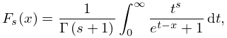
Antia (1993) gives minimax rational approximations for $\mathrm{\Gamma }\left(s+1\right)F_s(x)$, where $F_s(x)$ is the Fermi–Dirac integral (25.12.14), for the intervals and , with $s=-\frac{1}{2},\frac{1}{2},\frac{3}{2},\frac{5}{2}$. For each $s$ there are three sets of approximations, with relative maximum errors ${10}^{-4},{10}^{-8},{10}^{-12}$.