Bessel transform
(0.008 seconds)
11—20 of 54 matching pages
11: 10.22 Integrals
…
►
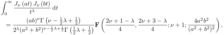
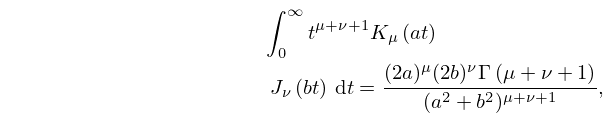
10.22.57
.
►
10.22.58
, .
…
►
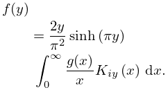
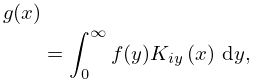
§10.22(v) Hankel Transform
►The Hankel transform (or Bessel transform) of a function is defined as … ►
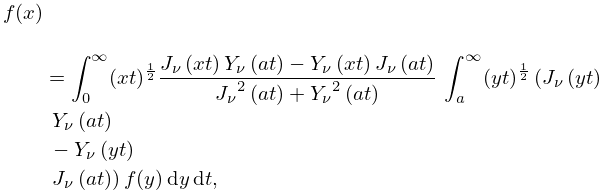
10.22.78
.
…
12: 13.23 Integrals
…
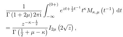
►
13.23.6
.
►
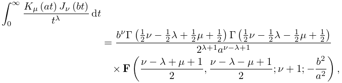
13.23.7
.
…
►For additional Hankel transforms and also other Bessel transforms see Erdélyi et al. (1954b, §8.18) and Oberhettinger (1972, §1.16 and 3.4.42–46, 4.4.45–47, 5.94–97).
…
13: Bibliography C
…
►
An algorithm for the Fourier-Bessel transform.
Comput. Phys. Comm. 23 (4), pp. 343–353.
…
►
Derivatives with respect to the degree and order of associated Legendre functions for using modified Bessel functions.
Integral Transforms Spec. Funct. 21 (7-8), pp. 581–588.
…
14: 10.43 Integrals
…
►
10.43.26
.
…
►
10.43.27
.
…
►
§10.43(v) Kontorovich–Lebedev Transform
… ►
10.43.30
…
►
10.43.31
…
15: 1.14 Integral Transforms
§1.14 Integral Transforms
…16: 18.17 Integrals
…
►
18.17.18
…
17: Bibliography P
…
►
Bounds for ratios of modified Bessel functions.
Integral Transform. Spec. Funct. 9 (4), pp. 293–298.
…
18: 3.5 Quadrature
…
►
Example. Laplace Transform Inversion
…19: 10.42 Zeros
…
►Properties of the zeros of and may be deduced from those of and , respectively, by application of the transformations (10.27.6) and (10.27.8).
…
