Bézier curves

SearchAdvancedHelp

(0.001 seconds)

11—20 of 48 matching pages

11: 27.19 Methods of Computation: Factorization

… ►Type I probabilistic algorithms include the Brent–Pollard rho algorithm (also called Monte Carlo method), the Pollard $p-1$ algorithm, and the Elliptic Curve Method (ecm). …

12: 31.8 Solutions via Quadratures

… ►The variables $\lambda$ and $\nu$ are two coordinates of the associated hyperelliptic (spectral) curve $\mathrm{\Gamma }:{\nu }^2={\prod }_{j=1}^{2g+1}(\lambda -{\lambda }_j)$. … ►The curve $\mathrm{\Gamma }$ reflects the finite-gap property of Equation (31.2.1) when the exponent parameters satisfy (31.8.1) for $m_j\in \mathbb{Z}$. …

13: 28.32 Mathematical Applications

… ►Also let $ℒ$ be a curve (possibly improper) such that the quantity … ►

28.32.6 $$w(z)={\int }_{ℒ}K(z,\zeta )u(\zeta )d\zeta$$

ⓘ

Symbols:

$dx$: differential of $x$ , $\int$: integral, $z$: complex variable, $\zeta$: variable, $u(\zeta )$: solution, $K(z,\zeta )$: solution and $ℒ$: curve

Permalink:

http://dlmf.nist.gov/28.32.E6

Encodings:

pMML, png, TeX

See also:

Annotations for §28.32(i), §28.32 and Ch.28

►defines a solution of Mathieu’s equation, provided that (in the case of an improper curve) the integral converges with respect to $z$ uniformly on compact subsets of $ℂ$. …

14: 1.6 Vectors and Vector-Valued Functions

… ►The geometrical image $C$ of a path $𝐜$ is called a simple closed curve if $𝐜$ is one-to-one, with the exception $𝐜(a)=𝐜(b)$. The curve $C$ is piecewise differentiable if $𝐜$ is piecewise differentiable. … … ►and $S$ be the closed and bounded point set in the $(x,y)$ plane having a simple closed curve $C$ as boundary. … ►

1.6.44 $${\iint }_S\left(\frac{\partial F_2}{\partial x}-\frac{\partial F_1}{\partial y}\right)dA={\int }_C𝐅\cdot d𝐬={\int }_C{F}_{1}dx+F_{2}dy.$$

ⓘ

Symbols:

$dx$: differential of $x$ , $\int$: integral, $\frac{\partial f}{\partial x}$: partial derivative of $f$ with respect to $x$ , $\partial x$: partial differential of $x$ , $𝐅(x,y)$: vector, $S$: closed region, $C$: closed curve and $F_j$: vector function components

Referenced by:

§1.6(iv)

Permalink:

http://dlmf.nist.gov/1.6.E44

Encodings:

pMML, png, TeX

See also:

Annotations for §1.6(iv), §1.6(iv), §1.6 and Ch.1

…

15: 32.3 Graphics

… ►

►►

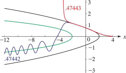
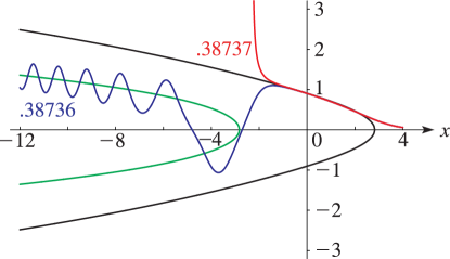
Figure 32.3.8: $u_k(x;\frac{1}{2})$ for $-12\le x\le 4$ with $k=0.47442$, $0.47443$. …The curves $u^2+\frac{1}{3}x\pm \frac{1}{6}\sqrt{x^2+12}=0$ are shown in green and black, respectively. Magnify

►

►►

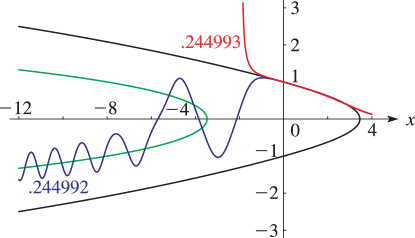
Figure 32.3.9: $u_k(x;\frac{3}{2})$ for $-12\le x\le 4$ with $k=0.38736$, $0.38737$. …The curves $u^2+\frac{1}{3}x\pm \frac{1}{6}\sqrt{x^2+24}=0$ are shown in green and black, respectively. Magnify

►

►►

Figure 32.3.10: $u_k(x;\frac{5}{2})$ for $-12\le x\le 4$ with $k=\mathrm{0.24499\hspace{0.33em}2}$, $\mathrm{0.24499\hspace{0.33em}3}$. …The curves $u^2+\frac{1}{3}x\pm \frac{1}{6}\sqrt{x^2+36}=0$ are shown in green and black, respectively. Magnify

16: 36.5 Stokes Sets

… ►The Stokes set is itself a cusped curve, connected to the cusp of the bifurcation set: … ►For $z=0$, the set consists of the two curves … ►In Figures 36.5.1–36.5.6 the plane is divided into regions by the dashed curves (Stokes sets) and the continuous curves (bifurcation sets). …

17: Philip J. Davis

… ►Moreover, a cutting plane feature allows users to track curves of intersection produced as a moving plane cuts through the function surface. …

18: 21.4 Graphics

… ►This Riemann matrix originates from the Riemann surface represented by the algebraic curve ${\mu }^3-{\lambda }^7+2{\lambda }^3\mu =0$; compare §21.7(i). … ►

►

►

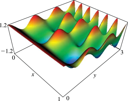
Figure 21.4.5: The real part of a genus 3 scaled Riemann theta function: $\mathrm{\Re }\widehat{\theta }\left(x+\mathrm{i}y,0,0\right|{𝛀}_2)$, $0\le x\le 1$, $0\le y\le 3$. This Riemann matrix originates from the genus 3 Riemann surface represented by the algebraic curve ${\mu }^3+2\mu -{\lambda }^4=0$; compare §21.7(i). Magnify 3D Help

19: 36.7 Zeros

… ►Inside the cusp, that is, for , the zeros form pairs lying in curved rows. … ►The zeros of these functions are curves in $𝐱=(x,y,z)$ space; see Nye (2007) for ${\mathrm{\Phi }}_3$ and Nye (2006) for ${\mathrm{\Phi }}^{(\mathrm{H})}$.

20: Preface

… ►Saunders was responsible for mesh generation for curves and surfaces, data computation and validation, graphics production, and interactive Web visualization. …