Askey polynomials

SearchAdvancedHelp

(0.004 seconds)

11—20 of 44 matching pages

11: Bibliography Z

… ►

Weighted derangements and the linearization coefficients of orthogonal Sheffer polynomials. Proc. London Math. Soc. (3) 65 (1), pp. 1–22.

ⓘ

External Links:

ISSN 0024-6115, Document, Link, MathReview (R. A. Askey), ZentralBlatt

Referenced by:

§18.18(v).

Encodings:

BibTeX

… ►

“Hidden symmetry” of Askey-Wilson polynomials. Theoret. and Math. Phys. 89 (2), pp. 1146–1157.

ⓘ

External Links:

MathReview (Vadim B. Kuznetsov), ZentralBlatt

Referenced by:

§18.38(iii).

Encodings:

BibTeX

…

12: Errata

… ►

18.28.1 $$p_n(x)=p_n(x;a,b,c,d|q)=a^{-n}\sum _{\mathrm{\ell }=0}^n{q}^{\mathrm{\ell }}{(ab{q}^{\mathrm{\ell }},ac{q}^{\mathrm{\ell }},ad{q}^{\mathrm{\ell }};q)}_{n-\mathrm{\ell }}\frac{{(q^{-n},abcd{q}^{n-1};q)}_{\mathrm{\ell }}}{{(q;q)}_{\mathrm{\ell }}}\prod _{j=0}^{\mathrm{\ell }-1}(1-2a{q}^{j}x+a^2{q}^{2j}),$$

18.28.1_5 $$R_n(z)=R_n(z;a,b,c,d|q)=\frac{p_n(\frac{1}{2}(z+z^{-1});a,b,c,d|q)}{a^{-n}{(ab,ac,ad;q)}_n}={}_4{}^{}\varphi _3^{}(\genfrac{}{}{0pt}{}{q^{-n},abcd{q}^{n-1},az,a{z}^{-1}}{ab,ac,ad};q,q)$$

Previously we presented all the information of these formulas in one equation

$$p_n(\cos \theta )=p_n(\cos \theta ;a,b,c,d|q)=a^{-n}\sum _{\mathrm{\ell }=0}^n{q}^{\mathrm{\ell }}{(ab{q}^{\mathrm{\ell }},ac{q}^{\mathrm{\ell }},ad{q}^{\mathrm{\ell }};q)}_{n-\mathrm{\ell }}\frac{{(q^{-n},abcd{q}^{n-1};q)}_{\mathrm{\ell }}}{{(q;q)}_{\mathrm{\ell }}}\prod _{j=0}^{\mathrm{\ell }-1}(1-2a{q}^j\cos \theta +a^2{q}^{2j})=a^{-n}{(ab,ac,ad;q)}_n{}_4{}^{}\varphi _3^{}(\genfrac{}{}{0pt}{}{q^{-n},abcd{q}^{n-1},a{\mathrm{e}}^{\mathrm{i}\theta },a{\mathrm{e}}^{-\mathrm{i}\theta }}{ab,ac,ad};q,q).$$

…

13: 18.30 Associated OP’s

… ►However, if the recurrence coefficients are polynomial, or rational, functions of $n$, polynomials of degree $n$ may be well defined for $c\in ℝ$ provided that $A_{n+c}{B}_{n+c}\ne 0,n=0,1,\mathrm{\dots }$ Askey and Wimp (1984). … ►

18.30.17 $${\int }_{-\mathrm{\infty }}^{\mathrm{\infty }}{𝒫}_n^{\lambda }(x;\varphi ,c){𝒫}_m^{\lambda }(x;\varphi ,c)w^{(\lambda )}(x,\varphi ,c)dx=\frac{\mathrm{\Gamma }\left(n+c+2\lambda \right)\mathrm{\Gamma }\left(c+1\right)}{{\left(c+1\right)}_n}{\delta }_{n,m},$$ or ,

ⓘ

Symbols:

$\mathrm{\Gamma }\left(z\right)$: gamma function, ${\delta }_{j,k}$: Kronecker delta, ${\left(a\right)}_n$: Pochhammer’s symbol (or shifted factorial), ${𝒫}_n^{\lambda }(x;\varphi ,c)$: associated Meixner–Pollaczek polynomial, $\pi$: the ratio of the circumference of a circle to its diameter, $dx$: differential of $x$ , $\int$: integral, $w(x)$: weight function, $m$: nonnegative integer, $n$: nonnegative integer and $x$: real variable

Sources:

Askey and Wimp (1984, (1.9)); Pollaczek (1950, formula following (16))

Permalink:

http://dlmf.nist.gov/18.30.E17

Encodings:

pMML, png, TeX

See also:

Annotations for §18.30(v), §18.30 and Ch.18

… ►

18.30.19 $$L_n^{\lambda }(x;c)=\underset{\varphi \to 0}{lim}{𝒫}_n^{(\lambda +1)/2}(\frac{-x}{2\sin \varphi };\varphi ,c),$$

ⓘ

Symbols:

$L_n^{\lambda }(x;c)$: associated Laguerre polynomial, ${𝒫}_n^{\lambda }(x;\varphi ,c)$: associated Meixner–Pollaczek polynomial, $\sin z$: sine function, $n$: nonnegative integer and $x$: real variable

Proof sketch:

Using the limit will convert (18.30.16) into (18.30.9). See also Askey and Wimp (1984, §2).

Permalink:

http://dlmf.nist.gov/18.30.E19

Encodings:

pMML, png, TeX

See also:

Annotations for §18.30(v), §18.30 and Ch.18

… ►

18.30.20 $$H_n(x;c)={\left(c+1\right)}_n\underset{\lambda \to \mathrm{\infty }}{lim}{\lambda }^{-n/2}{𝒫}_n^{\lambda }(x{\lambda }^{1/2};\pi /2,c).$$

ⓘ

Symbols:

${\left(a\right)}_n$: Pochhammer’s symbol (or shifted factorial), $H_n(x;c)$: associated Hermite polynomial, ${𝒫}_n^{\lambda }(x;\varphi ,c)$: associated Meixner–Pollaczek polynomial, $\pi$: the ratio of the circumference of a circle to its diameter, $n$: nonnegative integer and $x$: real variable

Proof sketch:

Using the limit will convert (18.30.16) into (18.30.13). See also Askey and Wimp (1984, §4).

Permalink:

http://dlmf.nist.gov/18.30.E20

Encodings:

pMML, png, TeX

See also:

Annotations for §18.30(v), §18.30 and Ch.18

… ►For associated Askey–Wilson polynomials see Rahman (2001). …

14: Bibliography N

… ►

Askey-Wilson polynomials: an affine Hecke algebra approach. In Laredo Lectures on Orthogonal Polynomials and Special Functions, Adv. Theory Spec. Funct. Orthogonal Polynomials, pp. 111–144.

ⓘ

External Links:

MathReview (V. L. Deshpande), ZentralBlatt

Referenced by:

§18.38(iii).

Encodings:

BibTeX

…

15: 18.35 Pollaczek Polynomials

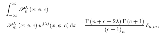
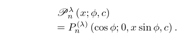
… ►The three types of Pollaczek polynomials were successively introduced in Pollaczek (1949a, b, 1950), see also Erdélyi et al. (1953b, p.219) and, for type 1 and 2, Szegö (1950) and Askey (1982b). … ►

18.35.10 $${𝒫}_n^{\lambda }(x;\varphi ,c)=P_n^{(\lambda )}(\cos \varphi ;0,x\sin \varphi ,c).$$

ⓘ

Symbols:

$Q_n^{(\lambda )}(x;a,b,c)$: Pollaczek polynomial, ${𝒫}_n^{\lambda }(x;\varphi ,c)$: associated Meixner–Pollaczek polynomial, $\cos z$: cosine function, $\sin z$: sine function, $n$: nonnegative integer and $x$: real variable

Source:

Askey and Wimp (1984)

Referenced by:

§18.30(v), §18.35(iii), Erratum (V1.2.0) Section 18.35

Permalink:

http://dlmf.nist.gov/18.35.E10

Encodings:

pMML, png, TeX

Addition (effective with 1.2.0):

This equation was added.

See also:

Annotations for §18.35(iii), §18.35 and Ch.18

… ►See Szegő (1975, Appendix, §§ 1–5), Askey (1982b), and Ismail (2009, §§ 5.4–5.5) for further results on type 2 Pollaczek polynomials. …

16: 18.4 Graphics

… ►

►►

Figure 18.4.1: Jacobi polynomials $P_n^{(1.5,-0.5)}\left(x\right)$, $n=1,2,3,4,5$. Magnify

►

►►

Figure 18.4.2: Jacobi polynomials $P_n^{(1.25,0.75)}\left(x\right)$, $n=7,8$. …See also Askey (1990). Magnify

… ►

►►

Figure 18.4.4: Legendre polynomials $P_n\left(x\right)$, $n=1,2,3,4,5$. Magnify

… ►

►►

Figure 18.4.7: Monic Hermite polynomials $h_n(x)=2^{-n}{H}_n\left(x\right)$, $n=1,2,3,4,5$. Magnify

…

17: 18.37 Classical OP’s in Two or More Variables

… ►In one variable they are essentially ultraspherical, Jacobi, continuous $q$-ultraspherical, or Askey–Wilson polynomials. …

18: Bibliography C

… ►

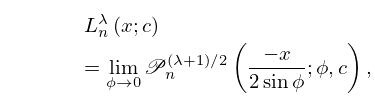
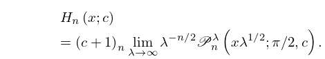
Asymptotic behaviour of the zeros of the (generalized) Laguerre polynomial $L_n^{\alpha }(x)$ as the index $\alpha \to \mathrm{\infty }$ and limiting formula relating Laguerre polynomials of large index and large argument to Hermite polynomials. Lett. Nuovo Cimento (2) 23 (3), pp. 101–102.

ⓘ

External Links:

ISSN 0024-1318, Document, MathReview (R. A. Askey)

Referenced by:

§18.7(iii).

Encodings:

BibTeX

… ►

Work Group of Computational Mathematics, University of Kassel, Germany.

ⓘ

Notes:

Computer Algebra and Orthogonal Polynomials: a Web service using Maple for online generation of formulas and graphs of orthogonal polynomials belonging to the Askey scheme. For further information see Swarttouw (1997) and Koepf (1999).

External Links:

CAOP

Referenced by:

1st item.

Encodings:

BibTeX

… ►

On the zeros of the Askey-Wilson polynomials, with applications to coding theory. SIAM J. Math. Anal. 18 (1), pp. 191–207.

ⓘ

External Links:

ISSN 0036-1410, Document, MathReview (Mourad E. H. Ismail), ZentralBlatt

Referenced by:

§18.38(iii).

Encodings:

BibTeX

…

19: 18.19 Hahn Class: Definitions

§18.19 Hahn Class: Definitions

►The Askey scheme extends the three families of classical OP’s (Jacobi, Laguerre and Hermite) with eight further families of OP’s for which the role of the differentiation operator $\frac{d}{dx}$ in the case of the classical OP’s is played by a suitable difference operator. …In addition to the limit relations in §18.7(iii) there are limit relations involving the further families in the Askey scheme, see §§18.21(ii) and 18.26(ii). The Askey scheme, depicted in Figure 18.21.1, gives a graphical representation of these limits. … ►Tables 18.19.1 and 18.19.2 provide definitions via orthogonality and standardization (§§18.2(i), 18.2(iii)) for the Hahn polynomials $Q_n(x;\alpha ,\beta ,N)$, Krawtchouk polynomials $K_n(x;p,N)$, Meixner polynomials $M_n(x;\beta ,c)$, and Charlier polynomials $C_n(x;a)$. …

20: Bibliography I

… ►

On polynomials orthogonal with respect to certain Sobolev inner products. J. Approx. Theory 65 (2), pp. 151–175.

ⓘ

External Links:

ISSN 0021-9045, Document, MathReview (R. A. Askey), ZentralBlatt

Referenced by:

§18.36(ii).

Encodings:

BibTeX

… ►

$q$-Hermite polynomials, biorthogonal rational functions, and $q$-beta integrals. Trans. Amer. Math. Soc. 346 (1), pp. 63–116.

ⓘ

External Links:

ISSN 0002-9947, FullText, MathReview (R. A. Askey), ZentralBlatt

Referenced by:

§18.28(vii).

Encodings:

BibTeX

… ►

Asymptotics of the Askey-Wilson and $q$-Jacobi polynomials. SIAM J. Math. Anal. 17 (6), pp. 1475–1482.

ⓘ

External Links:

ISSN 0036-1410, Document, MathReview (David M. Bressoud), ZentralBlatt

Referenced by:

§18.29.

Encodings:

BibTeX

… ►

Classical and Quantum Orthogonal Polynomials in One Variable. Encyclopedia of Mathematics and its Applications, Vol. 98, Cambridge University Press, Cambridge.

ⓘ

Notes:

With two chapters by Walter Van Assche, With a foreword by Richard A. Askey, Corrected reprint of the 2005 original.

External Links:

ISBN 978-0-521-14347-9, MathReview Entry, ZentralBlatt

Referenced by:

§18.12, (18.15.4_5), (18.16.19), (18.16.20), (18.16.21), §18.17(ii), §18.18(vii), §18.19, (18.2.20), §18.2(vi), §18.2(xii), §18.2(xii), §18.2(x), §18.20(i), §18.20(ii), §18.21(ii), §18.22(i), §18.22(ii), §18.22(iii), §18.23, §18.25(i), §18.25(iii), §18.26(i), §18.26(iv), (18.27.4), §18.27(i), §18.27(ii), §18.27(iii), §18.27(v), §18.27(vi), §18.28(i), §18.28(ii), §18.28(iii), §18.28(v), §18.28(vi), §18.28(vii), §18.28(viii), §18.30(vi), §18.30(vii), §18.30(iii), §18.30(iv), §18.30, §18.30(vi), §18.34(i), §18.34(ii), §18.34(ii), §18.34(iii), (18.35.4), (18.35.5), (18.35.6), (18.35.6_2), (18.35.6_3), (18.35.6_4), (18.35.7), (18.35.8), §18.35(ii), §18.35(iii), §18.36(iii), §18.38(ii), §18.39(iv), §18.39(iv), §18.39(iv), (18.40.4), Profile Mourad E.H. Ismail, Erratum (V1.0.20) for Chapter 18 Orthogonal Polynomials.

Encodings:

BibTeX

…