/shop/%E2%99%9F%F0%9F%AA%90%F0%9F%A6%B8%20Buy%20DNP%20Online%20$0.99%20Per%20Capsule%3A%20%F0%9F%92%A3%20www.BuyDNPOnline.cc%20%F0%9F%92%A3%20Buy%20DNP%20UK%20%F0%9F%A6%B8%F0%9F%AA%90%E2%99%9F%20Buy%20DNP%20In%20Australia%20-%20Buy%20DNP-www.BuyDNPOnline.cc

SearchAdvancedHelp

Did you mean /shop/%E2%99%9F%F0%9F%AA%90%F0%9F%A6%B8%20Buy%20DNP%20Online%20$0.99%20Per%20Capsule%3A%20%F0%9F%92%A3%20www.BuyDNPOnline.cc%20%F0%9F%92%A3%20Buy%20DNP%20UK%20%F0%9F%A6%B8%F0%9F%AA%90%E2%99%9F%20Buy%20DNP%20In%20Australia%20-%20Buy%20DNP-www.feshbachpublishing.com ?

(0.038 seconds)

1—10 of 983 matching pages

1: 34.6 Definition: $\mathit{9}j$ Symbol

§34.6 Definition: $\mathit{9}j$ Symbol

►The $\mathit{9}j$ symbol may be defined either in terms of $\mathit{3}j$ symbols or equivalently in terms of $\mathit{6}j$ symbols: ►

34.6.1

ⓘ

Defines:

: $\mathit{9}j$ symbol

Symbols:

: $\mathit{3}j$ symbol, $j,j_r$: non-negative integers or non-negative integers plus one half., $r$: nonnegative integer and $s$: integer

Permalink:

http://dlmf.nist.gov/34.6.E1

Encodings:

pMML, png, TeX

See also:

Annotations for §34.6 and Ch.34

►

34.6.2

ⓘ

Symbols:

: $\mathit{9}j$ symbol, : $\mathit{6}j$ symbol and $j,j_r$: non-negative integers or non-negative integers plus one half.

Referenced by:

§34.13

Permalink:

http://dlmf.nist.gov/34.6.E2

Encodings:

pMML, png, TeX

See also:

Annotations for §34.6 and Ch.34

►The $\mathit{9}j$ symbol may also be written as a finite triple sum equivalent to a terminating generalized hypergeometric series of three variables with unit arguments. …

2: 34.13 Methods of Computation

§34.13 Methods of Computation

►Methods of computation for $\mathit{3}j$ and $\mathit{6}j$ symbols include recursion relations, see Schulten and Gordon (1975a), Luscombe and Luban (1998), and Edmonds (1974, pp. 42–45, 48–51, 97–99); summation of single-sum expressions for these symbols, see Varshalovich et al. (1988, §§8.2.6, 9.2.1) and Fang and Shriner (1992); evaluation of the generalized hypergeometric functions of unit argument that represent these symbols, see Srinivasa Rao and Venkatesh (1978) and Srinivasa Rao (1981). ►For $\mathit{9}j$ symbols, methods include evaluation of the single-sum series (34.6.2), see Fang and Shriner (1992); evaluation of triple-sum series, see Varshalovich et al. (1988, §10.2.1) and Srinivasa Rao et al. (1989). A review of methods of computation is given in Srinivasa Rao and Rajeswari (1993, Chapter VII, pp. 235–265). …

3: 16.7 Relations to Other Functions

… ►For $\mathit{3}j$, $\mathit{6}j$, $\mathit{9}j$ symbols see Chapter 34. Further representations of special functions in terms of ${}_p{}^{}F_q^{}$ functions are given in Luke (1969a, §§6.2–6.3), and an extensive list of ${}_{q+1}{}^{}F_q^{}$ functions with rational numbers as parameters is given in Krupnikov and Kölbig (1997).

4: 15.3 Graphics

… ►

►►

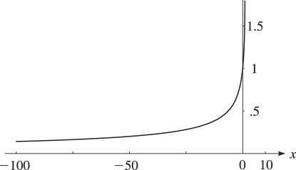
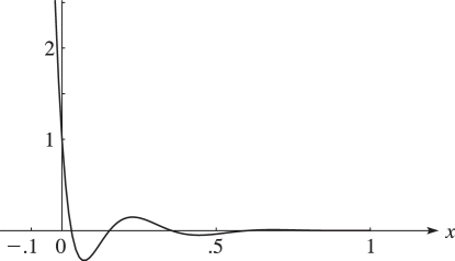
Figure 15.3.1: $F(\frac{4}{3},\frac{9}{16};\frac{14}{5};x),-100\le x\le 1$. Magnify

►

►►

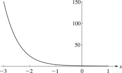
Figure 15.3.2: $F(5,-10;1;x),-0.023\le x\le 1$. Magnify

►

►►

Figure 15.3.3: $F(1,-10;10;x),-3\le x\le 1$. Magnify

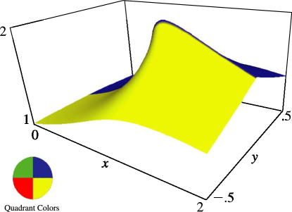
… ►In Figures 15.3.5 and 15.3.6, height corresponds to the absolute value of the function and color to the phase. … ►

►

►

Figure 15.3.5: $F(\frac{4}{3},\frac{9}{16};\frac{14}{5};x+\mathrm{i}y),0\le x\le 2,-0.5\le y\le 0.5$. … Magnify 3D Help

…

5: 19.9 Inequalities

… ►Throughout this subsection , except in (19.9.4). … ►Even for the extremely eccentric ellipse with $a=99$ and $b=1$, this is correct within 0. … ►Sharper inequalities for $F(\varphi ,k)$ are: … ►Inequalities for both $F(\varphi ,k)$ and $E(\varphi ,k)$ involving inverse circular or inverse hyperbolic functions are given in Carlson (1961b, §4). … ►Other inequalities for $F(\varphi ,k)$ can be obtained from inequalities for $R_F(x,y,z)$ given in Carlson (1966, (2.15)) and Carlson (1970) via (19.25.5).

6: 16.24 Physical Applications

… ►Generalized hypergeometric functions and Appell functions appear in the evaluation of the so-called Watson integrals which characterize the simplest possible lattice walks. … ►

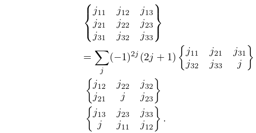
§16.24(iii) $\mathit{3}j$, $\mathit{6}j$, and $\mathit{9}j$ Symbols

… ►They can be expressed as ${}_3{}^{}F_2^{}$ functions with unit argument. …These are balanced ${}_4{}^{}F_3^{}$ functions with unit argument. Lastly, special cases of the $\mathit{9}j$ symbols are ${}_5{}^{}F_4^{}$ functions with unit argument. …

7: Bibliography T

… ►

On the connection formula for the first Painlevé equation—from the viewpoint of the exact WKB analysis. Sūrikaisekikenkyūsho Kōkyūroku (931), pp. 70–99.

ⓘ

Notes:

Painlevé functions and asymptotic analysis (Japanese) (Kyoto, 1995)

External Links:

FullText, MathReview (Andrei A. Kapaev)

Referenced by:

§32.12(i).

Encodings:

BibTeX

… ►

LSFBTR: A subroutine for calculating spherical Bessel transforms. Comput. Phys. Comm. 30 (1), pp. 93–99.

ⓘ

Notes:

Single-precision Fortran.

External Links:

ISSN 0010-4655, Document, Code

Referenced by:

9th item.

Encodings:

BibTeX

… ►

Algorithm 926: incomplete gamma functions with negative arguments. ACM Trans. Math. Software 39 (2), pp. Art. 14, 9.

ⓘ

External Links:

ISSN 0098-3500, Document, FullText, MathReview Entry, ZentralBlatt

Referenced by:

7th item, §8.28(ii).

Encodings:

BibTeX

… ►

Angular Momentum: An Illustrated Guide to Rotational Symmetries for Physical Systems. A Wiley-Interscience Publication, John Wiley & Sons Inc., New York.

ⓘ

Notes:

With 1 Macintosh floppy disk (3.5 inch; DD). Programs for the calculation of $3j,6j,9j$ symbols are included.

External Links:

ISBN 0-471-55264-X, MathReview (J. F. Cornwell), ZentralBlatt

Referenced by:

§34.3(vii).

Encodings:

BibTeX

… ►

Theory of the Fresnel integral. USSR Comput. Math. and Math. Phys. 9 (4), pp. 271–279.

ⓘ

Notes:

Translation of the paper in Zh. Vychisl. Mat. Mat. Fiz., Vol. 9, No. 4, 938-944, 1969

External Links:

Document, ZentralBlatt

Referenced by:

§7.13(iv).

Encodings:

BibTeX

8: 34.12 Physical Applications

§34.12 Physical Applications

►The angular momentum coupling coefficients ($\mathit{3}j$, $\mathit{6}j$, and $\mathit{9}j$ symbols) are essential in the fields of nuclear, atomic, and molecular physics. For applications in nuclear structure, see de-Shalit and Talmi (1963); in atomic spectroscopy, see Biedenharn and van Dam (1965, pp. 134–200), Judd (1998), Sobelman (1992, Chapter 4), Shore and Menzel (1968, pp. 268–303), and Wigner (1959); in molecular spectroscopy and chemical reactions, see Burshtein and Temkin (1994, Chapter 5), and Judd (1975). $\mathit{3}j,\mathit{6}j$, and $\mathit{9}j$ symbols are also found in multipole expansions of solutions of the Laplace and Helmholtz equations; see Carlson and Rushbrooke (1950) and Judd (1976).

9: Publications

… ►

Design of a Digital Mathematical Library for Science, Technology and Education, Proceedings of the IEEE Forum on Research and Technology Advances in Digital Libraries (IEEE ADL ’99, Baltimore, Maryland, May 19, 1999).

►

Using Numerical Grid Generation to Facilitate 3D Visualization of Complicated Mathematical Functions, Technical Report NISTIR 6413 (November 1999), National Institute of Standards and Technology.

… ►

The DLMF Project: A New Initiative in Classical Special Functions, in Special Functions—Proceedings of the International Workshop, Hong Kong, June 21-25, 1999 (C. Dunkl, M. Ismail, R. Wong, eds.), World Scientific, pp. 207–220.

… ►

Technical Aspects of the Digital Library of Mathematical Functions, Annals of Mathematics and Artificial Intelligence—Special Issue on Mathematical Knowledge Management, Vol. 38, Nos. 1–3, pp. 121–136.

… ►

NIST’s Digital Library of Mathematial Functions, Physics Today 71, 2, 48 (2018), pp. 48–53.

10: Bibliography

… ►

Some determinants of Bernoulli, Euler and related numbers. Portugal. Math. 18, pp. 91–99.

ⓘ

External Links:

FullText, MathReview (D. P. Banerjee), ZentralBlatt

Referenced by:

§24.14(ii).

Encodings:

BibTeX

… ►

Applications of basic hypergeometric functions. SIAM Rev. 16 (4), pp. 441–484.

ⓘ

External Links:

Document, MathReview (L. J. Slater), ZentralBlatt

Referenced by:

§17.16, Ch.17.

Encodings:

BibTeX

… ►

Theorems on generalized Dedekind sums. Pacific J. Math. 2 (1), pp. 1–9.

ⓘ

External Links:

MathReview (N. G. de Bruijn), ZentralBlatt

Referenced by:

(25.11.41), (25.11.42), §25.11(xii).

Encodings:

BibTeX

… ►

Numerical Tables for Angular Correlation Computations in $\alpha$-, $\beta$- and $\gamma$-Spectroscopy: $3j$-, $6j$-, $9j$-Symbols, F- and $\mathrm{\Gamma }$-Coefficients. Landolt-Börnstein Numerical Data and Functional Relationships in Science and Technology, Springer-Verlag.

ⓘ

External Links:

ISBN 978-3-540-04218-1

Referenced by:

§34.14.

Encodings:

BibTeX

… ►

A new treatment of the ellipsoidal wave equation. Proc. London Math. Soc. (3) 9, pp. 21–50.

ⓘ

External Links:

ISSN 0024-6115, Document, MathReview (J. Meixner), ZentralBlatt

Referenced by:

§29.11.

Encodings:

BibTeX

…