.2022%E5%B9%B4%E8%B6%B3%E7%90%83%E4%B8%96%E7%95%8C%E6%9D%AF%E5%86%A0%E5%86%9B_%E3%80%8E%E7%BD%91%E5%9D%80%3A68707.vip%E3%80%8F%E8%B6%B3%E7%90%83%E6%AF%94%E8%B5%9B%E8%B5%8C%E7%94%A8%E4%BB%80%E4%B9%88app_b5p6v3_2022%E5%B9%B412%E6%9C%882%E6%97%A56%E6%97%B627%E5%88%8638%E7%A7%92_3xvvl7r9d.cc

SearchAdvancedHelp

Did you mean .2022%E5%B9%B4%E8%B6%B3%E7%90%83%E4%B8%96%E7%95%8C%E6%9D%AF%E5%86%A0%E5%86%9B_%E3%80%8E%E7%BD%91%E5%9D%80%3A68707.vip%E3%80%8F%E8%B6%B3%E7%90%83%E6%AF%94%E8%B5%9B%E8%B5%8C%E7%94%A8%E4%BB%80%E4%B9%88app_b5p6v3_2022%E5%B9%412%E6%9C%882%E6%97%256%E6%97%627%E5%88%86384%E7%A7%92_3xvvl7r9d.cc ?

(0.048 seconds)

1—10 of 743 matching pages

1: 9.2 Differential Equation

… ►

9.2.2 $$w=\mathrm{Ai}\left(z\right),\mathrm{Bi}\left(z\right),\mathrm{Ai}\left(z{\mathrm{e}}^{\mp 2\pi \mathrm{i}/3}\right).$$

ⓘ

Symbols:

$\mathrm{Ai}\left(z\right)$: Airy function, $\mathrm{Bi}\left(z\right)$: Airy function, $\pi$: the ratio of the circumference of a circle to its diameter, $\mathrm{e}$: base of natural logarithm, $\mathrm{i}$: imaginary unit, $z$: complex variable and $w$: ODE solution

Source:

Olver (1997b, pp. 392–393, 413–414)

Permalink:

http://dlmf.nist.gov/9.2.E2

Encodings:

pMML, png, TeX

See also:

Annotations for §9.2(i), §9.2 and Ch.9

… ►

9.2.3 $$\mathrm{Ai}\left(0\right)=\frac{1}{3^{2/3}\mathrm{\Gamma }\left(\frac{2}{3}\right)}=\mathrm{0.35502\hspace{0.33em}80538}\mathrm{\dots },$$

ⓘ

Symbols:

$\mathrm{Ai}\left(z\right)$: Airy function and $\mathrm{\Gamma }\left(z\right)$: gamma function

Source:

Olver (1997b, (1.03), p. 392)

A&S Ref:

10.4.4 (with more digits)

Permalink:

http://dlmf.nist.gov/9.2.E3

Encodings:

pMML, png, TeX

See also:

Annotations for §9.2(ii), §9.2 and Ch.9

►

9.2.4 $${\mathrm{Ai}}^{\prime }\left(0\right)=-\frac{1}{3^{1/3}\mathrm{\Gamma }\left(\frac{1}{3}\right)}=-\mathrm{0.25881\hspace{0.33em}94037}\mathrm{\dots },$$

ⓘ

Symbols:

$\mathrm{Ai}\left(z\right)$: Airy function and $\mathrm{\Gamma }\left(z\right)$: gamma function

Source:

Olver (1997b, (1.03), p. 392)

A&S Ref:

10.4.5 (with more digits)

Permalink:

http://dlmf.nist.gov/9.2.E4

Encodings:

pMML, png, TeX

See also:

Annotations for §9.2(ii), §9.2 and Ch.9

►

9.2.5 $$\mathrm{Bi}\left(0\right)=\frac{1}{3^{1/6}\mathrm{\Gamma }\left(\frac{2}{3}\right)}=\mathrm{0.61492\hspace{0.33em}66274}\mathrm{\dots },$$

ⓘ

Symbols:

$\mathrm{Bi}\left(z\right)$: Airy function and $\mathrm{\Gamma }\left(z\right)$: gamma function

Source:

Olver (1997b, (1.11), p. 393)

A&S Ref:

10.4.4 (in different form)

Referenced by:

(9.12.15)

Permalink:

http://dlmf.nist.gov/9.2.E5

Encodings:

pMML, png, TeX

See also:

Annotations for §9.2(ii), §9.2 and Ch.9

►

9.2.6 $${\mathrm{Bi}}^{\prime }\left(0\right)=\frac{3^{1/6}}{\mathrm{\Gamma }\left(\frac{1}{3}\right)}=\mathrm{0.44828\hspace{0.33em}83573}\mathrm{\dots }.$$

ⓘ

Symbols:

$\mathrm{Bi}\left(z\right)$: Airy function and $\mathrm{\Gamma }\left(z\right)$: gamma function

Source:

Olver (1997b, (1.11), p. 393)

A&S Ref:

10.4.5 (in different form)

Referenced by:

(9.12.15)

Permalink:

http://dlmf.nist.gov/9.2.E6

Encodings:

pMML, png, TeX

See also:

Annotations for §9.2(ii), §9.2 and Ch.9

…

2: 19.37 Tables

… ►Tabulated for $\varphi =0(5^{\circ }){90}^{\circ }$, $k^2=0(.01)1$ to 10D by Fettis and Caslin (1964). ►Tabulated for $\varphi =0(1^{\circ }){90}^{\circ }$, $k^2=0(.01)1$ to 7S by Beli͡akov et al. (1962). … ►Tabulated for $\varphi =0(5^{\circ }){90}^{\circ }$, $k=0(.01)1$ to 10D by Fettis and Caslin (1964). ►Tabulated for $\varphi =0(5^{\circ }){90}^{\circ }$, $\arcsin k=0(1^{\circ }){90}^{\circ }$ to 6D by Byrd and Friedman (1971), for $\varphi =0(5^{\circ }){90}^{\circ }$, $\arcsin k=0(2^{\circ }){90}^{\circ }$ and $5^{\circ }({10}^{\circ }){85}^{\circ }$ to 8D by Abramowitz and Stegun (1964, Chapter 17), and for $\varphi =0({10}^{\circ }){90}^{\circ }$, $\arcsin k=0(5^{\circ }){90}^{\circ }$ to 9D by Zhang and Jin (1996, pp. 674–675). … ►Tabulated (with different notation) for $\varphi =0({15}^{\circ }){90}^{\circ }$, ${\alpha }^2=0(.1)1$, $\arcsin k=0({15}^{\circ }){90}^{\circ }$ to 5D by Abramowitz and Stegun (1964, Chapter 17), and for $\varphi =0({15}^{\circ }){90}^{\circ }$, ${\alpha }^2=0(.1)1$, $\arcsin k=0({15}^{\circ }){90}^{\circ }$ to 7D by Zhang and Jin (1996, pp. 676–677). …

3: 20.15 Tables

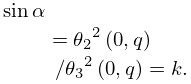
… ►This reference gives ${\theta }_j(x,q)$, $j=1,2,3,4$, and their logarithmic $x$-derivatives to 4D for $x/\pi =0(.1)1$, $\alpha =0(9^{\circ }){90}^{\circ }$, where $\alpha$ is the modular angle given by ►

20.15.1 $$\sin \alpha ={\theta }_2^2(0,q)/{\theta }_3^2(0,q)=k.$$

ⓘ

Defines:

$\alpha$: modular angle (locally)

Symbols:

${\theta }_j(z,q)$: theta function, $\sin z$: sine function and $q$: nome

Referenced by:

§20.15, §20.15

Permalink:

http://dlmf.nist.gov/20.15.E1

Encodings:

pMML, png, TeX

See also:

Annotations for §20.15 and Ch.20

►Spenceley and Spenceley (1947) tabulates ${\theta }_1(x,q)/{\theta }_2(0,q)$, ${\theta }_2(x,q)/{\theta }_2(0,q)$, ${\theta }_3(x,q)/{\theta }_4(0,q)$, ${\theta }_4(x,q)/{\theta }_4(0,q)$ to 12D for $u=0(1^{\circ }){90}^{\circ }$, $\alpha =0(1^{\circ }){89}^{\circ }$, where $u=2x/(\pi {\theta }_3^2(0,q))$ and $\alpha$ is defined by (20.15.1), together with the corresponding values of ${\theta }_2(0,q)$ and ${\theta }_4(0,q)$. ►Lawden (1989, pp. 270–279) tabulates ${\theta }_j(x,q)$, $j=1,2,3,4$, to 5D for $x=0(1^{\circ }){90}^{\circ }$, $q=0.1(.1)0.9$, and also $q$ to 5D for $k^2=0(.01)1$. ►Tables of Neville’s theta functions ${\theta }_s(x,q)$, ${\theta }_c(x,q)$, ${\theta }_d(x,q)$, ${\theta }_n(x,q)$ (see §20.1) and their logarithmic $x$-derivatives are given in Abramowitz and Stegun (1964, pp. 582–585) to 9D for $\epsilon ,\alpha =0(5^{\circ }){90}^{\circ }$, where (in radian measure) $\epsilon =x/{\theta }_3^2(0,q)=\pi x/(2K\left(k\right))$, and $\alpha$ is defined by (20.15.1). …

4: 5.16 Sums

… ►

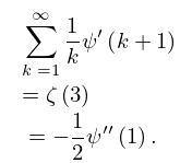
5.16.1 $$\sum _{k=1}^{\mathrm{\infty }}{(-1)}^k{\psi }^{\prime }\left(k\right)=-\frac{{\pi }^2}{8},$$

ⓘ

Symbols:

$\pi$: the ratio of the circumference of a circle to its diameter, $\psi \left(z\right)$: psi (or digamma) function and $k$: nonnegative integer

Permalink:

http://dlmf.nist.gov/5.16.E1

Encodings:

pMML, png, TeX

See also:

Annotations for §5.16 and Ch.5

►

5.16.2 $$\sum _{k=1}^{\mathrm{\infty }}\frac{1}{k}{\psi }^{\prime }\left(k+1\right)=\zeta \left(3\right)=-\frac{1}{2}{\psi }^{\prime \prime }\left(1\right).$$

ⓘ

Symbols:

$\zeta \left(s\right)$: Riemann zeta function, $\psi \left(z\right)$: psi (or digamma) function and $k$: nonnegative integer

Permalink:

http://dlmf.nist.gov/5.16.E2

Encodings:

pMML, png, TeX

See also:

Annotations for §5.16 and Ch.5

… ►For sums of gamma functions see Andrews et al. (1999, Chapters 2 and 3) and §§15.2(i), 16.2. ►For related sums involving finite field analogs of the gamma and beta functions (Gauss and Jacobi sums) see Andrews et al. (1999, Chapter 1) and Terras (1999, pp. 90, 149).

5: 14.33 Tables

… ►

Abramowitz and Stegun (1964, Chapter 8) tabulates ${𝖯}_n\left(x\right)$ for $n=0(1)3,9,10$, $x=0(.01)1$, 5–8D; ${𝖯}_n^{\prime }\left(x\right)$ for $n=1(1)4,9,10$, $x=0(.01)1$, 5–7D; ${𝖰}_n\left(x\right)$ and ${𝖰}_n^{\prime }\left(x\right)$ for $n=0(1)3,9,10$, $x=0(.01)1$, 6–8D; $P_n\left(x\right)$ and $P_n^{\prime }\left(x\right)$ for $n=0(1)5,9,10$, $x=1(.2)10$, 6S; $Q_n\left(x\right)$ and $Q_n^{\prime }\left(x\right)$ for $n=0(1)3,9,10$, $x=1(.2)10$, 6S. (Here primes denote derivatives with respect to $x$.)

►

Zhang and Jin (1996, Chapter 4) tabulates ${𝖯}_n\left(x\right)$ for $n=2(1)5,10$, $x=0(.1)1$, 7D; ${𝖯}_n\left(\cos \theta \right)$ for $n=1(1)4,10$, $\theta =0(5^{\circ }){90}^{\circ }$, 8D; ${𝖰}_n\left(x\right)$ for $n=0(1)2,10$, $x=0(.1)0.9$, 8S; ${𝖰}_n\left(\cos \theta \right)$ for $n=0(1)3,10$, $\theta =0(5^{\circ }){90}^{\circ }$, 8D; ${𝖯}_n^m\left(x\right)$ for $m=1(1)4$, $n-m=0(1)2$, $n=10$, $x=0,0.5$, 8S; ${𝖰}_n^m\left(x\right)$ for $m=1(1)4$, $n=0(1)2,10$, 8S; ${𝖯}_{\nu }^m\left(\cos \theta \right)$ for $m=0(1)3$, $\nu =0(.25)5$, $\theta =0({15}^{\circ }){90}^{\circ }$, 5D; $P_n\left(x\right)$ for $n=2(1)5,10$, $x=1(1)10$, 7S; $Q_n\left(x\right)$ for $n=0(1)2,10$, $x=2(1)10$, 8S. Corresponding values of the derivative of each function are also included, as are 6D values of the first 5 $\nu$-zeros of ${𝖯}_{\nu }^m\left(\cos \theta \right)$ and of its derivative for $m=0(1)4$, $\theta ={10}^{\circ },{30}^{\circ },{150}^{\circ }$.

►

Belousov (1962) tabulates ${𝖯}_n^m\left(\cos \theta \right)$ (normalized) for $m=0(1)36$, $n-m=0(1)56$, $\theta =0({2.5}^{\circ }){90}^{\circ }$, 6D.

…

6: 33.26 Software

… ►

Noble (2004). Fortran 90.

…

7: Bibliography E

… ►

Some recent results on the zeros of Bessel functions and orthogonal polynomials. J. Comput. Appl. Math. 133 (1-2), pp. 65–83.

ⓘ

External Links:

ISSN 0377-0427, Document, MathReview (N. Hayek Calil), ZentralBlatt

Referenced by:

§10.21(iv).

Encodings:

BibTeX

… ►

The Fuchsian equation of second order with four singularities. Duke Math. J. 9 (1), pp. 48–58.

ⓘ

External Links:

Document, MathReview (R. E. Langer), ZentralBlatt

Referenced by:

§31.11(i).

Encodings:

BibTeX

… ►

Algorithm 934: Fortran 90 subroutines to compute Mathieu functions for complex values of the parameter. ACM Trans. Math. Softw. 40 (1), pp. 8:1–8:19.

ⓘ

External Links:

ISSN 0098-3500, FullText, Document, MathReview Entry, ZentralBlatt

Referenced by:

4th item, §28.36(iii).

Encodings:

BibTeX

►

Algorithm 861: Fortran 90 subroutines for computing the expansion coefficients of Mathieu functions using Blanch’s algorithm. ACM Trans. Math. Software 32 (4), pp. 622–634.

ⓘ

External Links:

ISSN 0098-3500, Document, FullText, MathReview Entry, ZentralBlatt

Referenced by:

3rd item, §28.36(iii).

Encodings:

BibTeX

… ►

On the representations of a number as a sum of three squares. Proc. London Math. Soc. (3) 9, pp. 575–594.

ⓘ

External Links:

Document, MathReview (S. Chowla), ZentralBlatt

Referenced by:

§20.12(i).

Encodings:

BibTeX

…

8: 27.2 Functions

… ►

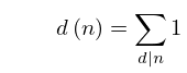
27.2.9 $$d\left(n\right)=\sum _{d|n}1$$

ⓘ

Symbols:

$d_k\left(n\right)$: divisor function, $d$: positive integer and $n$: positive integer

A&S Ref:

24.3.3 I.A

Permalink:

http://dlmf.nist.gov/27.2.E9

Encodings:

pMML, png, TeX

See also:

Annotations for §27.2(i), §27.2 and Ch.27

… ►It is the special case $k=2$ of the function $d_k\left(n\right)$ that counts the number of ways of expressing $n$ as the product of $k$ factors, with the order of factors taken into account. …Note that ${\sigma }_0\left(n\right)=d\left(n\right)$. … ►Table 27.2.2 tabulates the Euler totient function $\varphi \left(n\right)$, the divisor function $d\left(n\right)$ ($={\sigma }_0(n)$), and the sum of the divisors $\sigma (n)$ ($={\sigma }_1(n)$), for $n=1(1)52$. … ►

Table 27.2.2: Functions related to division.

► ►►►

$n$	$\varphi \left(n\right)$	$d\left(n\right)$	$\sigma \left(n\right)$	$n$	$\varphi \left(n\right)$	$d\left(n\right)$	$\sigma \left(n\right)$	$n$	$\varphi \left(n\right)$	$d\left(n\right)$	$\sigma \left(n\right)$	$n$	$\varphi \left(n\right)$	$d\left(n\right)$	$\sigma \left(n\right)$
1	1	1	1	14	6	4	24	27	18	4	40	40	16	8	90
…

►

9: 27.20 Methods of Computation: Other Number-Theoretic Functions

… ►See Calkin et al. (2007), and Lehmer (1941, pp. 5–83). …

10: 4.48 Software

… ►

Kearfott (1996). Fortran 90.

…