DLMF: Untitled Document

… ►

Functions $K\left(k\right)$ and $E\left(k\right)$

►Tabulated for

k^{2}=0(.01)1

to 6D by Byrd and Friedman (1971), to 15D for

K\left(k\right)

and 9D for

E\left(k\right)

by Abramowitz and Stegun (1964, Chapter 17), and to 10D by Fettis and Caslin (1964). ►Tabulated for

k=0(.01)1

to 10D by Fettis and Caslin (1964), and for

k=0(.02)1

to 7D by Zhang and Jin (1996, p. 673). … ►Tabulated for

\phi=5^{\circ}(5^{\circ})80^{\circ}(2.5^{\circ})90^{\circ}

,

\alpha^{2}=-1(.1)-0.1,0.1(.1)1

,

k^{2}=0(.05)0.9(.02)1

to 10D by Fettis and Caslin (1964) (and warns of inaccuracies in Selfridge and Maxfield (1958) and Paxton and Rollin (1959)). ►Tabulated for

\phi=0(1^{\circ})90^{\circ}

,

\alpha^{2}=0(.05)0.85,0.88(.02)0.94(.01)0.98(.005)1

,

k^{2}=0(.01)1

to 7S by Beli͡akov et al. (1962). …

… ►

•

Blanch and Clemm (1962) includes values of ${\operatorname{Mc}^{(1)}_{n}}\left(x,\sqrt{q}\right)$ and ${\operatorname{Mc}^{(1)}_{n}}'\left(x,\sqrt{q}\right)$ for $n=0(1)15$ with $q=0(.05)1$ , $x=0(.02)1$ . Also ${\operatorname{Ms}^{(1)}_{n}}\left(x,\sqrt{q}\right)$ and ${\operatorname{Ms}^{(1)}_{n}}'\left(x,\sqrt{q}\right)$ for $n=1(1)15$ with $q=0(.05)1$ , $x=0(.02)1$ . Precision is generally 7D.

►

•

Blanch and Clemm (1965) includes values of ${\operatorname{Mc}^{(2)}_{n}}\left(x,\sqrt{q}\right)$ , ${\operatorname{Mc}^{(2)}_{n}}'\left(x,\sqrt{q}\right)$ for $n=0(1)7$ , $x=0(.02)1$ ; $n=8(1)15$ , $x=0(.01)1$ . Also ${\operatorname{Ms}^{(2)}_{n}}\left(x,\sqrt{q}\right)$ , ${\operatorname{Ms}^{(2)}_{n}}'\left(x,\sqrt{q}\right)$ for $n=1(1)7$ , $x=0(.02)1$ ; $n=8(1)15$ , $x=0(.01)1$ . In all cases $q=0(.05)1$ . Precision is generally 7D. Approximate formulas and graphs are also included.

… ►

•

National Bureau of Standards (1967) includes the eigenvalues $a_{n}\left(q\right)$ , $b_{n}\left(q\right)$ for $n=0(1)3$ with $q=0(.2)20(.5)37(1)100$ , and $n=4(1)15$ with $q=0(2)100$ ; Fourier coefficients for $\operatorname{ce}_{n}\left(x,q\right)$ and $\operatorname{se}_{n}\left(x,q\right)$ for $n=0(1)15$ , $n=1(1)15$ , respectively, and various values of $q$ in the interval $[0,100]$ ; joining factors $g_{\mathit{e},n}(\sqrt{q})$ , $f_{\mathit{e},n}(\sqrt{q})$ for $n=0(1)15$ with $q=0(.5\mbox{ to }10)100$ (but in a different notation). Also, eigenvalues for large values of $q$ . Precision is generally 8D.

… ►

•

Zhang and Jin (1996, pp. 521–532) includes the eigenvalues $a_{n}\left(q\right)$ , $b_{n+1}\left(q\right)$ for $n=0(1)4$ , $q=0(1)50$ ; $n=0(1)20$ ( $a$ ’s) or 19 ( $b$ ’s), $q=1,3,5,10,15,25,50(50)200$ . Fourier coefficients for $\operatorname{ce}_{n}\left(x,10\right)$ , $\operatorname{se}_{n+1}\left(x,10\right)$ , $n=0(1)7$ . Mathieu functions $\operatorname{ce}_{n}\left(x,10\right)$ , $\operatorname{se}_{n+1}\left(x,10\right)$ , and their first $x$ -derivatives for $n=0(1)4$ , $x=0(5^{\circ})90^{\circ}$ . Modified Mathieu functions ${\operatorname{Mc}^{(j)}_{n}}\left(x,\sqrt{10}\right)$ , ${\operatorname{Ms}^{(j)}_{n+1}}\left(x,\sqrt{10}\right)$ , and their first $x$ -derivatives for $n=0(1)4$ , $j=1,2$ , $x=0(.2)4$ . Precision is mostly 9S.

… ►

•

Zhang and Jin (1996, pp. 533–535) includes the zeros (in degrees) of $\operatorname{ce}_{n}\left(x,10\right)$ , $\operatorname{se}_{n}\left(x,10\right)$ for $n=1(1)10$ , and the first 5 zeros of ${\operatorname{Mc}^{(j)}_{n}}\left(x,\sqrt{10}\right)$ , ${\operatorname{Ms}^{(j)}_{n}}\left(x,\sqrt{10}\right)$ for $n=0$ or $1(1)8$ , $j=1,2$ . Precision is mostly 9S.

…

… ►

•

Abramowitz and Stegun (1964) tabulates: $\zeta\left(n\right)$ , $n=2,3,4,\dots$ , 20D (p. 811); $\operatorname{Li}_{2}\left(1-x\right)$ , $x=0(.01)0.5$ , 9D (p. 1005); $f(\theta)$ , $\theta=15^{\circ}(1^{\circ})30^{\circ}(2^{\circ})90^{\circ}(5^{\circ})180^{\circ}$ , $f(\theta)+\theta\ln\theta$ , $\theta=0(1^{\circ})15^{\circ}$ , 6D (p. 1006). Here $f(\theta)$ denotes Clausen’s integral, given by the right-hand side of (25.12.9).

►

•

Morris (1979) tabulates $\operatorname{Li}_{2}\left(x\right)$ (§25.12(i)) for $\pm x=0.02(.02)1(.1)6$ to 30D.

►

•

Cloutman (1989) tabulates $\Gamma\left(s+1\right)F_{s}(x)$ , where $F_{s}(x)$ is the Fermi–Dirac integral (25.12.14), for $s=-\frac{1}{2},\frac{1}{2},\frac{3}{2},\frac{5}{2}$ , $x=-5(.05)25$ , to 12S.

…

… ►

•

Abramowitz and Stegun (1964, Chapter 7) includes $\operatorname{erf}x$ , $(2/\sqrt{\pi})e^{-x^{2}}$ , $x\in[0,2]$ , 10D; $(2/\sqrt{\pi})e^{-x^{2}}$ , $x\in[2,10]$ , 8S; $xe^{x^{2}}\operatorname{erfc}x$ , $x^{-2}\in[0,0.25]$ , 7D; $2^{n}\Gamma\left(\frac{1}{2}n+1\right)\mathop{\mathrm{i}^{n}\mathrm{erfc}}% \left(x\right)$ , $n=1(1)6,10,11$ , $x\in[0,5]$ , 6S; $F\left(x\right)$ , $x\in[0,2]$ , 10D; $xF\left(x\right)$ , $x^{-2}\in[0,0.25]$ , 9D; $C\left(x\right)$ , $S\left(x\right)$ , $x\in[0,5]$ , 7D; $\mathrm{f}\left(x\right)$ , $\mathrm{g}\left(x\right)$ , $x\in[0,1]$ , $x^{-1}\in[0,1]$ , 15D.

►

•

Abramowitz and Stegun (1964, Table 27.6) includes the Goodwin–Staton integral $G\left(x\right)$ , $x=1(.1)3(.5)8$ , 4D; also $G\left(x\right)+\ln x$ , $x=0(.05)1$ , 4D.

… ►

•

Zhang and Jin (1996, pp. 637, 639) includes $(2/\sqrt{\pi})e^{-x^{2}}$ , $\operatorname{erf}x$ , $x=0(.02)1(.04)3$ , 8D; $C\left(x\right)$ , $S\left(x\right)$ , $x=0(.2)10(2)100(100)500$ , 8D.

… ►

•

Abramowitz and Stegun (1964, Chapter 7) includes $w\left(z\right)$ , $x=0(.1)3.9$ , $y=0(.1)3$ , 6D.

… ►

•

Zhang and Jin (1996, p. 642) includes the first 10 zeros of $\operatorname{erf}z$ , 9D; the first 25 distinct zeros of $C\left(z\right)$ and $S\left(z\right)$ , 8S.

… ►

•

Žurina and Osipova (1964) tabulates $M\left(a,b,x\right)$ and $U\left(a,b,x\right)$ for $b=2$ , $a=-0.98(.02)1.10$ , $x=0(.01)4$ , 7D or 7S.

…

… ►

•

Miller (1946) tabulates $\operatorname{Ai}\left(x\right)$ , $\operatorname{Ai}'\left(x\right)$ for $x=-20(.01)2;$ $\operatorname{log}_{10}\operatorname{Ai}\left(x\right)$ , $\operatorname{Ai}'\left(x\right)/\operatorname{Ai}\left(x\right)$ for $x=0(.1)25(1)75$ ; $\operatorname{Bi}\left(x\right)$ , $\operatorname{Bi}'\left(x\right)$ for $x=-10(.1)2.5$ ; $\operatorname{log}_{10}\operatorname{Bi}\left(x\right)$ , $\operatorname{Bi}'\left(x\right)/\operatorname{Bi}\left(x\right)$ for $x=0(.1)10$ ; $M\left(x\right)$ , $N\left(x\right)$ , $\theta\left(x\right)$ , $\phi\left(x\right)$ (respectively $F(x)$ , $G(x)$ , $\chi(x)$ , $\psi(x)$ ) for $x=-80(1)-30(.1)0$ . Precision is generally 8D; slightly less for some of the auxiliary functions. Extracts from these tables are included in Abramowitz and Stegun (1964, Chapter 10), together with some auxiliary functions for large arguments.

►

•

Fox (1960, Table 3) tabulates $2\pi^{1/2}x^{1/4}\*\exp(\tfrac{2}{3}x^{3/2})\*\operatorname{Ai}\left(x\right)$ , $2\pi^{1/2}x^{-1/4}\*\exp(\tfrac{2}{3}x^{3/2})\*\operatorname{Ai}'\left(x\right)$ , $\pi^{1/2}x^{1/4}\*\exp(-\tfrac{2}{3}x^{3/2})\*\operatorname{Bi}\left(x\right)$ , and $\pi^{1/2}x^{-1/4}\*\exp(-\tfrac{2}{3}x^{3/2})\*\operatorname{Bi}'\left(x\right)$ for $\tfrac{3}{2}x^{-3/2}=0(.001)0.05$ , together with similar auxiliary functions for negative values of $x$ . Precision is 10D.

… ►

•

Yakovleva (1969) tabulates Fock’s functions $U(x)\equiv\sqrt{\pi}\operatorname{Bi}\left(x\right)$ , $U^{\prime}(x)=\sqrt{\pi}\operatorname{Bi}'\left(x\right)$ , $V(x)\equiv\sqrt{\pi}\operatorname{Ai}\left(x\right)$ , $V^{\prime}(x)=\sqrt{\pi}\operatorname{Ai}'\left(x\right)$ for $x=-9(.001)9$ . Precision is 7S.

… ►

•

National Bureau of Standards (1958) tabulates $A_{0}(x)\equiv\pi\operatorname{Hi}\left(-x\right)$ and $-A_{0}^{\prime}(x)\equiv\pi\operatorname{Hi}'\left(-x\right)$ for $x=0(.01)1(.02)5(.05)11$ and $1/x=0.01(.01)0.1$ ; $\int_{0}^{x}A_{0}(t)\,\mathrm{d}t$ for $x=0.5,1(1)11$ . Precision is 8D.

►

•

Nosova and Tumarkin (1965) tabulates $e_{0}(x)\equiv\pi\operatorname{Hi}\left(-x\right)$ , $e^{\prime}_{0}(x)=-\pi\operatorname{Hi}'\left(-x\right)$ , $\widetilde{e}_{0}(-x)\equiv-\pi\operatorname{Gi}\left(x\right)$ , $\widetilde{e}^{\mspace{2.0mu}\prime}_{0}(-x)=\pi\operatorname{Gi}'\left(x\right)$ for $x=-1(.01)10$ ; 7D. Also included are the real and imaginary parts of $e_{0}(z)$ and $ie^{\prime}_{0}(z)$ , where $z=iy$ and $y=0(.01)9$ ; 6-7D.

…

… ►

•

British Association for the Advancement of Science (1937) tabulates $J_{0}\left(x\right)$ , $J_{1}\left(x\right)$ , $x=0(.001)16(.01)25$ , 10D; $Y_{0}\left(x\right)$ , $Y_{1}\left(x\right)$ , $x=0.01(.01)25$ , 8–9S or 8D. Also included are auxiliary functions to facilitate interpolation of the tables of $Y_{0}\left(x\right)$ , $Y_{1}\left(x\right)$ for small values of $x$ , as well as auxiliary functions to compute all four functions for large values of $x$ .

… ►

•

Achenbach (1986) tabulates $J_{0}\left(x\right)$ , $J_{1}\left(x\right)$ , $Y_{0}\left(x\right)$ , $Y_{1}\left(x\right)$ , $x=0(.1)8$ , 20D or 18–20S.

… ►

•

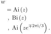
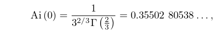
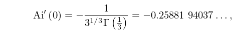
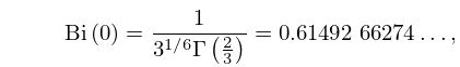
Abramowitz and Stegun (1964, Chapter 9) tabulates $j_{n,m}$ , $J_{n}'\left(j_{n,m}\right)$ , ${j^{\prime}_{n,m}}$ , $J_{n}\left({j^{\prime}_{n,m}}\right)$ , $n=0(1)8$ , $m=1(1)20$ , 5D (10D for $n=0$ ), $y_{n,m}$ , $Y_{n}'\left(y_{n,m}\right)$ , ${y^{\prime}_{n,m}}$ , $Y_{n}\left({y^{\prime}_{n,m}}\right)$ , $n=0(1)8$ , $m=1(1)20$ , 5D (8D for $n=0$ ), $J_{0}\left(j_{0,m}x\right)$ , $m=1(1)5$ , $x=0(.02)1$ , 5D. Also included are the first 5 zeros of the functions $xJ_{1}\left(x\right)-\lambda J_{0}\left(x\right)$ , $J_{1}\left(x\right)-\lambda xJ_{0}\left(x\right)$ , $J_{0}\left(x\right)Y_{0}\left(\lambda x\right)-Y_{0}\left(x\right)J_{0}\left(% \lambda x\right)$ , $J_{1}\left(x\right)Y_{1}\left(\lambda x\right)-Y_{1}\left(x\right)J_{1}\left(% \lambda x\right)$ , $J_{1}\left(x\right)Y_{0}\left(\lambda x\right)-Y_{1}\left(x\right)J_{0}\left(% \lambda x\right)$ for various values of $\lambda$ and $\lambda^{-1}$ in the interval $[0,1]$ , 4–8D.

… ►

•

Makinouchi (1966) tabulates all values of $j_{\nu,m}$ and $y_{\nu,m}$ in the interval $(0,100)$ , with at least 29S. These are for $\nu=0(1)5$ , 10, 20; $\nu=\tfrac{3}{2}$ , $\tfrac{5}{2}$ ; $\nu=m/n$ with $m=1(1)n-1$ and $n=3(1)8$ , except for $\nu=\tfrac{1}{2}$ .

… ►

•

Achenbach (1986) tabulates $I_{0}\left(x\right)$ , $I_{1}\left(x\right)$ , $K_{0}\left(x\right)$ , $K_{1}\left(x\right)$ , $x=0(.1)8$ , 19D or 19–21S.

…

… ►

9.2.2

w=\operatorname{Ai}\left(z\right),\;\operatorname{Bi}\left(z\right),\;% \operatorname{Ai}\left(ze^{\mp 2\pi\mathrm{i}/3}\right).

ⓘ

Symbols:: $\operatorname{Ai}\left(\NVar{z}\right)$ : Airy function, $\operatorname{Bi}\left(\NVar{z}\right)$ : Airy function, $\pi$ : the ratio of the circumference of a circle to its diameter, $\mathrm{e}$ : base of natural logarithm, $\mathrm{i}$ : imaginary unit, $z$ : complex variable and $w$ : ODE solution
Source:: Olver (1997b, pp. 392–393, 413–414)
Permalink:: http://dlmf.nist.gov/9.2.E2
Encodings:: pMML, png, TeX
See also:: Annotations for §9.2(i), §9.2 and Ch.9

… ►

9.2.3

\operatorname{Ai}\left(0\right)=\frac{1}{3^{2/3}\Gamma\left(\tfrac{2}{3}\right% )}=0.35502\;80538\ldots,

ⓘ

Symbols:: $\operatorname{Ai}\left(\NVar{z}\right)$ : Airy function and $\Gamma\left(\NVar{z}\right)$ : gamma function
Source:: Olver (1997b, (1.03), p. 392)
A&S Ref:: 10.4.4 (with more digits)
Permalink:: http://dlmf.nist.gov/9.2.E3
Encodings:: pMML, png, TeX
See also:: Annotations for §9.2(ii), §9.2 and Ch.9

►

9.2.4

\operatorname{Ai}'\left(0\right)=-\frac{1}{3^{1/3}\Gamma\left(\tfrac{1}{3}% \right)}=-0.25881\;94037\ldots,

ⓘ

Symbols:: $\operatorname{Ai}\left(\NVar{z}\right)$ : Airy function and $\Gamma\left(\NVar{z}\right)$ : gamma function
Source:: Olver (1997b, (1.03), p. 392)
A&S Ref:: 10.4.5 (with more digits)
Permalink:: http://dlmf.nist.gov/9.2.E4
Encodings:: pMML, png, TeX
See also:: Annotations for §9.2(ii), §9.2 and Ch.9

►

9.2.5

\operatorname{Bi}\left(0\right)=\frac{1}{3^{1/6}\Gamma\left(\tfrac{2}{3}\right% )}=0.61492\;66274\ldots,

ⓘ

Symbols:: $\operatorname{Bi}\left(\NVar{z}\right)$ : Airy function and $\Gamma\left(\NVar{z}\right)$ : gamma function
Source:: Olver (1997b, (1.11), p. 393)
A&S Ref:: 10.4.4 (in different form)
Referenced by:: (9.12.15)
Permalink:: http://dlmf.nist.gov/9.2.E5
Encodings:: pMML, png, TeX
See also:: Annotations for §9.2(ii), §9.2 and Ch.9

►

9.2.6

\operatorname{Bi}'\left(0\right)=\frac{3^{1/6}}{\Gamma\left(\tfrac{1}{3}\right% )}=0.44828\;83573\ldots.

ⓘ

Symbols:: $\operatorname{Bi}\left(\NVar{z}\right)$ : Airy function and $\Gamma\left(\NVar{z}\right)$ : gamma function
Source:: Olver (1997b, (1.11), p. 393)
A&S Ref:: 10.4.5 (in different form)
Referenced by:: (9.12.15)
Permalink:: http://dlmf.nist.gov/9.2.E6
Encodings:: pMML, png, TeX
See also:: Annotations for §9.2(ii), §9.2 and Ch.9

…

§34.6 Definition: $\mathit{9j}$ Symbol

►The

\mathit{9j}

symbol may be defined either in terms of

\mathit{3j}

symbols or equivalently in terms of

\mathit{6j}

symbols: ►

34.6.1

\begin{Bmatrix}j_{11}&j_{12}&j_{13}\\ j_{21}&j_{22}&j_{23}\\ j_{31}&j_{32}&j_{33}\end{Bmatrix}=\sum_{\mbox{\scriptsize all }m_{rs}}\begin{% pmatrix}j_{11}&j_{12}&j_{13}\\ m_{11}&m_{12}&m_{13}\end{pmatrix}\begin{pmatrix}j_{21}&j_{22}&j_{23}\\ m_{21}&m_{22}&m_{23}\end{pmatrix}\begin{pmatrix}j_{31}&j_{32}&j_{33}\\ m_{31}&m_{32}&m_{33}\end{pmatrix}\*\begin{pmatrix}j_{11}&j_{21}&j_{31}\\ m_{11}&m_{21}&m_{31}\end{pmatrix}\begin{pmatrix}j_{12}&j_{22}&j_{32}\\ m_{12}&m_{22}&m_{32}\end{pmatrix}\begin{pmatrix}j_{13}&j_{23}&j_{33}\\ m_{13}&m_{23}&m_{33}\end{pmatrix},

ⓘ

Defines:: $\begin{Bmatrix}\NVar{j_{11}}&\NVar{j_{12}}&\NVar{j_{13}}\\ \NVar{j_{21}}&\NVar{j_{22}}&\NVar{j_{23}}\\ \NVar{j_{31}}&\NVar{j_{32}}&\NVar{j_{33}}\end{Bmatrix}$ : $\mathit{9j}$ symbol
Symbols:: $\begin{pmatrix}\NVar{j_{1}}&\NVar{j_{2}}&\NVar{j_{3}}\\ \NVar{m_{1}}&\NVar{m_{2}}&\NVar{m_{3}}\end{pmatrix}$ : $\mathit{3j}$ symbol, $j,j_{r}$ : non-negative integers or non-negative integers plus one half., $r$ : nonnegative integer and $s$ : integer
Permalink:: http://dlmf.nist.gov/34.6.E1
Encodings:: pMML, png, TeX
See also:: Annotations for §34.6 and Ch.34

►

34.6.2

\begin{Bmatrix}j_{11}&j_{12}&j_{13}\\ j_{21}&j_{22}&j_{23}\\ j_{31}&j_{32}&j_{33}\end{Bmatrix}=\sum_{j}(-1)^{2j}(2j+1)\begin{Bmatrix}j_{11}% &j_{21}&j_{31}\\ j_{32}&j_{33}&j\end{Bmatrix}\begin{Bmatrix}j_{12}&j_{22}&j_{32}\\ j_{21}&j&j_{23}\end{Bmatrix}\begin{Bmatrix}j_{13}&j_{23}&j_{33}\\ j&j_{11}&j_{12}\end{Bmatrix}.

ⓘ

Symbols:: $\begin{Bmatrix}\NVar{j_{11}}&\NVar{j_{12}}&\NVar{j_{13}}\\ \NVar{j_{21}}&\NVar{j_{22}}&\NVar{j_{23}}\\ \NVar{j_{31}}&\NVar{j_{32}}&\NVar{j_{33}}\end{Bmatrix}$ : $\mathit{9j}$ symbol, $\begin{Bmatrix}\NVar{j_{1}}&\NVar{j_{2}}&\NVar{j_{3}}\\ \NVar{l_{1}}&\NVar{l_{2}}&\NVar{l_{3}}\end{Bmatrix}$ : $\mathit{6j}$ symbol and $j,j_{r}$ : non-negative integers or non-negative integers plus one half.
Referenced by:: §34.13
Permalink:: http://dlmf.nist.gov/34.6.E2
Encodings:: pMML, png, TeX
See also:: Annotations for §34.6 and Ch.34

►The

\mathit{9j}

symbol may also be written as a finite triple sum equivalent to a terminating generalized hypergeometric series of three variables with unit arguments. …

… ►The integral for

E\left(\phi,k\right)

is well defined if

k^{2}={\sin}^{2}\phi=1

, and the Cauchy principal value (§1.4(v)) of

\Pi\left(\phi,\alpha^{2},k\right)

is taken if

1-\alpha^{2}{\sin}^{2}\phi

vanishes at an interior point of the integration path. … ►

§19.2(iv) A Related Function: $R_{C}\left(x,y\right)$

… ►Formulas involving

\Pi\left(\phi,\alpha^{2},k\right)

that are customarily different for circular cases, ordinary hyperbolic cases, and (hyperbolic) Cauchy principal values, are united in a single formula by using

R_{C}\left(x,y\right)

. … ►When

x

and

y

are positive,

R_{C}\left(x,y\right)

is an inverse circular function if

x<y

and an inverse hyperbolic function (or logarithm) if

x>y

: …For the special cases of

R_{C}\left(x,x\right)

and

R_{C}\left(0,y\right)

see (19.6.15). …

.02%E5%B9%B4%E4%B8%96%E7%95%8C%E6%9D%AF%E6%B2%99%E7%89%B9%E5%B0%8F%E7%BB%84%E8%B5%9B%E3%80%8E%E7%BD%91%E5%9D%80%3Amxsty.cc%E3%80%8F.%E4%B8%96%E7%95%8C%E6%9D%AF%E8%B6%B3%E5%BD%A9%E7%8E%A9%E6%B3%95%E8%A7%84%E5%88%99.m6q3s2-oeoo02w0g

1—10 of 737 matching pages

1: 19.37 Tables

Functions $K\left(k\right)$ and $E\left(k\right)$

2: 28.35 Tables

3: 25.19 Tables

4: 7.23 Tables

5: 13.30 Tables

6: 9.18 Tables

7: 10.75 Tables

8: 9.2 Differential Equation

9: 34.6 Definition: $\mathit{9j}$ Symbol

§34.6 Definition: $\mathit{9j}$ Symbol

10: 19.2 Definitions

§19.2(iv) A Related Function: $R_{C}\left(x,y\right)$

.02%E5%B9%B4%E4%B8%96%E7%95%8C%E6%9D%AF%E6%B2%99%E7%89%B9%E5%B0%8F%E7%BB%84%E8%B5%9B%E3%80%8E%E7%BD%91%E5%9D%80%3Amxsty.cc%E3%80%8F.%E4%B8%96%E7%95%8C%E6%9D%AF%E8%B6%B3%E5%BD%A9%E7%8E%A9%E6%B3%95%E8%A7%84%E5%88%99.m6q3s2-oeoo02w0g

1—10 of 737 matching pages

1: 19.37 Tables

Functions K ⁡ ( k ) and E ⁡ ( k )

2: 28.35 Tables

3: 25.19 Tables

4: 7.23 Tables

5: 13.30 Tables

6: 9.18 Tables

7: 10.75 Tables

8: 9.2 Differential Equation

9: 34.6 Definition: 9 ⁢ j Symbol

§34.6 Definition: 9 ⁢ j Symbol

10: 19.2 Definitions

§19.2(iv) A Related Function: R C ⁡ ( x , y )

Functions $K\left(k\right)$ and $E\left(k\right)$

9: 34.6 Definition: $\mathit{9j}$ Symbol

§34.6 Definition: $\mathit{9j}$ Symbol

§19.2(iv) A Related Function: $R_{C}\left(x,y\right)$