.%E9%9F%A9%E5%9B%BD%E5%85%B0%E8%8A%9D%E5%B2%9B%E4%B8%96%E7%95%8C%E6%9D%AF%E5%85%AC%E5%9B%AD_%E3%80%8E%E7%BD%91%E5%9D%80%3A68707.vip%E3%80%8F%E7%AF%AE%E7%90%83%E4%B8%96%E7%95%8C%E6%9D%AF%E7%AB%9E%E7%8C%9C_b5p6v3_pr7bnb1nb.com

The terms "a68707.vip", "pr7bnb1nb.com", "b5p6v3" were not found.Possible alternative terms: "caniuse.com", "8.17.vi".

(0.095 seconds)

1—10 of 848 matching pages

1: 34.6 Definition: $\mathit{9j}$ Symbol

§34.6 Definition: $\mathit{9j}$ Symbol

►The

\mathit{9j}

symbol may be defined either in terms of

\mathit{3j}

symbols or equivalently in terms of

\mathit{6j}

symbols: ►

34.6.1

\begin{Bmatrix}j_{11}&j_{12}&j_{13}\\ j_{21}&j_{22}&j_{23}\\ j_{31}&j_{32}&j_{33}\end{Bmatrix}=\sum_{\mbox{\scriptsize all }m_{rs}}\begin{% pmatrix}j_{11}&j_{12}&j_{13}\\ m_{11}&m_{12}&m_{13}\end{pmatrix}\begin{pmatrix}j_{21}&j_{22}&j_{23}\\ m_{21}&m_{22}&m_{23}\end{pmatrix}\begin{pmatrix}j_{31}&j_{32}&j_{33}\\ m_{31}&m_{32}&m_{33}\end{pmatrix}\*\begin{pmatrix}j_{11}&j_{21}&j_{31}\\ m_{11}&m_{21}&m_{31}\end{pmatrix}\begin{pmatrix}j_{12}&j_{22}&j_{32}\\ m_{12}&m_{22}&m_{32}\end{pmatrix}\begin{pmatrix}j_{13}&j_{23}&j_{33}\\ m_{13}&m_{23}&m_{33}\end{pmatrix},

ⓘ

Defines:: $\begin{Bmatrix}\NVar{j_{11}}&\NVar{j_{12}}&\NVar{j_{13}}\\ \NVar{j_{21}}&\NVar{j_{22}}&\NVar{j_{23}}\\ \NVar{j_{31}}&\NVar{j_{32}}&\NVar{j_{33}}\end{Bmatrix}$ : $\mathit{9j}$ symbol
Symbols:: $\begin{pmatrix}\NVar{j_{1}}&\NVar{j_{2}}&\NVar{j_{3}}\\ \NVar{m_{1}}&\NVar{m_{2}}&\NVar{m_{3}}\end{pmatrix}$ : $\mathit{3j}$ symbol, $j,j_{r}$ : non-negative integers or non-negative integers plus one half., $r$ : nonnegative integer and $s$ : integer
Permalink:: http://dlmf.nist.gov/34.6.E1
Encodings:: pMML, png, TeX
See also:: Annotations for §34.6 and Ch.34

►

34.6.2

\begin{Bmatrix}j_{11}&j_{12}&j_{13}\\ j_{21}&j_{22}&j_{23}\\ j_{31}&j_{32}&j_{33}\end{Bmatrix}=\sum_{j}(-1)^{2j}(2j+1)\begin{Bmatrix}j_{11}% &j_{21}&j_{31}\\ j_{32}&j_{33}&j\end{Bmatrix}\begin{Bmatrix}j_{12}&j_{22}&j_{32}\\ j_{21}&j&j_{23}\end{Bmatrix}\begin{Bmatrix}j_{13}&j_{23}&j_{33}\\ j&j_{11}&j_{12}\end{Bmatrix}.

ⓘ

Symbols:: $\begin{Bmatrix}\NVar{j_{11}}&\NVar{j_{12}}&\NVar{j_{13}}\\ \NVar{j_{21}}&\NVar{j_{22}}&\NVar{j_{23}}\\ \NVar{j_{31}}&\NVar{j_{32}}&\NVar{j_{33}}\end{Bmatrix}$ : $\mathit{9j}$ symbol, $\begin{Bmatrix}\NVar{j_{1}}&\NVar{j_{2}}&\NVar{j_{3}}\\ \NVar{l_{1}}&\NVar{l_{2}}&\NVar{l_{3}}\end{Bmatrix}$ : $\mathit{6j}$ symbol and $j,j_{r}$ : non-negative integers or non-negative integers plus one half.
Referenced by:: §34.13
Permalink:: http://dlmf.nist.gov/34.6.E2
Encodings:: pMML, png, TeX
See also:: Annotations for §34.6 and Ch.34

►The

\mathit{9j}

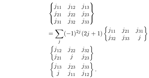
symbol may also be written as a finite triple sum equivalent to a terminating generalized hypergeometric series of three variables with unit arguments. …

2: 34.12 Physical Applications

§34.12 Physical Applications

►The angular momentum coupling coefficients (

\mathit{3j}

\mathit{6j}

, and

\mathit{9j}

symbols) are essential in the fields of nuclear, atomic, and molecular physics. …

\mathit{3j},\mathit{6j}

, and

\mathit{9j}

symbols are also found in multipole expansions of solutions of the Laplace and Helmholtz equations; see Carlson and Rushbrooke (1950) and Judd (1976).

3: 16.7 Relations to Other Functions

… ►For

\mathit{3j}

\mathit{6j}

\mathit{9j}

symbols see Chapter 34. Further representations of special functions in terms of

{{}_{p}F_{q}}

functions are given in Luke (1969a, §§6.2–6.3), and an extensive list of

{{}_{q+1}F_{q}}

functions with rational numbers as parameters is given in Krupnikov and Kölbig (1997).

4: 16.24 Physical Applications

… ►

§16.24(iii) $\mathit{3j}$ , $\mathit{6j}$ , and $\mathit{9j}$ Symbols

►The

\mathit{3j}

symbols, or Clebsch–Gordan coefficients, play an important role in the decomposition of reducible representations of the rotation group into irreducible representations. They can be expressed as

{{}_{3}F_{2}}

functions with unit argument. …These are balanced

{{}_{4}F_{3}}

functions with unit argument. Lastly, special cases of the

\mathit{9j}

symbols are

{{}_{5}F_{4}}

functions with unit argument. …

5: 9 Airy and Related Functions

Chapter 9 Airy and Related Functions

…

9: 16.10 Expansions in Series of ${{}_{p}F_{q}}$ Functions

§16.10 Expansions in Series of ${{}_{p}F_{q}}$ Functions

… ►

16.10.1

{{}_{p+r}F_{q+s}}\left({a_{1},\dots,a_{p},c_{1},\dots,c_{r}\atop b_{1},\dots,b% _{q},d_{1},\dots,d_{s}};z\zeta\right)=\sum_{k=0}^{\infty}\frac{{\left(\mathbf{% a}\right)_{k}}{\left(\alpha\right)_{k}}{\left(\beta\right)_{k}}(-z)^{k}}{{% \left(\mathbf{b}\right)_{k}}{\left(\gamma+k\right)_{k}}k!}{{}_{p+2}F_{q+1}}% \left({\alpha+k,\beta+k,a_{1}+k,\dots,a_{p}+k\atop\gamma+2k+1,b_{1}+k,\dots,b_% {q}+k};z\right){{}_{r+2}F_{s+2}}\left({-k,\gamma+k,c_{1},\dots,c_{r}\atop% \alpha,\beta,d_{1},\dots,d_{s}};\zeta\right).

ⓘ

Symbols:: ${{}_{\NVar{p}}F_{\NVar{q}}}\left(\NVar{a_{1},\dots,a_{p}};\NVar{b_{1},\dots,b_% {q}};\NVar{z}\right)$ or ${{}_{\NVar{p}}F_{\NVar{q}}}\left({\NVar{a_{1},\dots,a_{p}}\atop\NVar{b_{1},% \dots,b_{q}}};\NVar{z}\right)$ : alternatively ${{}_{\NVar{p}}F_{\NVar{q}}}\left(\NVar{\mathbf{a}};\NVar{\mathbf{b}};\NVar{z}\right)$ or ${{}_{\NVar{p}}F_{\NVar{q}}}\left({\NVar{\mathbf{a}}\atop\NVar{\mathbf{b}}};% \NVar{z}\right)$
generalized hypergeometric function, ${\left(\NVar{a}\right)_{\NVar{n}}}$ : Pochhammer’s symbol (or shifted factorial), $!$ : factorial (as in $n!$ ), $p$ : nonnegative integer, $q$ : nonnegative integer, $z$ : complex variable, $a,a_{1},\ldots,a_{p}$ : real or complex parameters and $b,b_{1},\ldots,b_{q}$ : real or complex parameters
Permalink:: http://dlmf.nist.gov/16.10.E1
Encodings:: pMML, png, TeX
See also:: Annotations for §16.10 and Ch.16

… ►

16.10.2

{{}_{p+1}F_{p}}\left({a_{1},\dots,a_{p+1}\atop b_{1},\dots,b_{p}};z\zeta\right% )=(1-z)^{-a_{1}}\sum_{k=0}^{\infty}\frac{{\left(a_{1}\right)_{k}}}{k!}{{}_{p+1% }F_{p}}\left({-k,a_{2},\dots,a_{p+1}\atop b_{1},\dots,b_{p}};\zeta\right)\left% (\frac{z}{z-1}\right)^{k}.

ⓘ

Symbols:: ${{}_{\NVar{p}}F_{\NVar{q}}}\left(\NVar{a_{1},\dots,a_{p}};\NVar{b_{1},\dots,b_% {q}};\NVar{z}\right)$ or ${{}_{\NVar{p}}F_{\NVar{q}}}\left({\NVar{a_{1},\dots,a_{p}}\atop\NVar{b_{1},% \dots,b_{q}}};\NVar{z}\right)$ : alternatively ${{}_{\NVar{p}}F_{\NVar{q}}}\left(\NVar{\mathbf{a}};\NVar{\mathbf{b}};\NVar{z}\right)$ or ${{}_{\NVar{p}}F_{\NVar{q}}}\left({\NVar{\mathbf{a}}\atop\NVar{\mathbf{b}}};% \NVar{z}\right)$
generalized hypergeometric function, ${\left(\NVar{a}\right)_{\NVar{n}}}$ : Pochhammer’s symbol (or shifted factorial), $!$ : factorial (as in $n!$ ), $p$ : nonnegative integer, $z$ : complex variable, $a,a_{1},\ldots,a_{p}$ : real or complex parameters and $b,b_{1},\ldots,b_{q}$ : real or complex parameters
Permalink:: http://dlmf.nist.gov/16.10.E2
Encodings:: pMML, png, TeX
See also:: Annotations for §16.10 and Ch.16

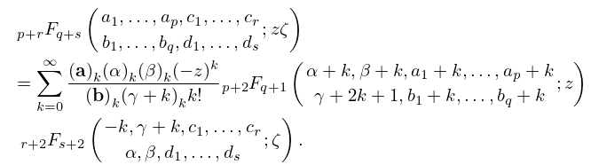
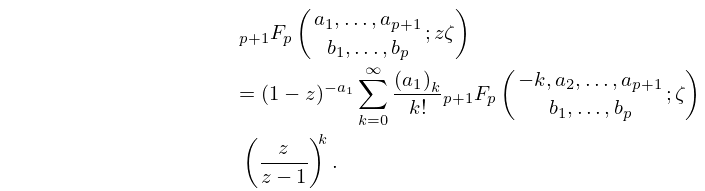
… ►Expansions of the form

\sum_{n=1}^{\infty}(\pm 1)^{n}{{}_{p}F_{p+1}}\left(\mathbf{a};\mathbf{b};-n^{2% }z^{2}\right)

are discussed in Miller (1997), and further series of generalized hypergeometric functions are given in Luke (1969b, Chapter 9), Luke (1975, §§5.10.2 and 5.11), and Prudnikov et al. (1990, §§5.3, 6.8–6.9).

10: 16.26 Approximations

… ►For discussions of the approximation of generalized hypergeometric functions and the Meijer

G

-function in terms of polynomials, rational functions, and Chebyshev polynomials see Luke (1975, §§5.12 - 5.13) and Luke (1977b, Chapters 1 and 9).

.%E9%9F%A9%E5%9B%BD%E5%85%B0%E8%8A%9D%E5%B2%9B%E4%B8%96%E7%95%8C%E6%9D%AF%E5%85%AC%E5%9B%AD_%E3%80%8E%E7%BD%91%E5%9D%80%3A68707.vip%E3%80%8F%E7%AF%AE%E7%90%83%E4%B8%96%E7%95%8C%E6%9D%AF%E7%AB%9E%E7%8C%9C_b5p6v3_pr7bnb1nb.com

1—10 of 848 matching pages

1: 34.6 Definition: $\mathit{9j}$ Symbol

§34.6 Definition: $\mathit{9j}$ Symbol

2: 34.12 Physical Applications

§34.12 Physical Applications

3: 16.7 Relations to Other Functions

4: 16.24 Physical Applications

§16.24(iii) $\mathit{3j}$ , $\mathit{6j}$ , and $\mathit{9j}$ Symbols

5: 9 Airy and Related Functions

Chapter 9 Airy and Related Functions

6: 15.3 Graphics

7: 34 3j, 6j, 9j Symbols

Chapter 34 $\mathit{3j},\mathit{6j},\mathit{9j}$ Symbols

8: 34.14 Tables

§34.14 Tables

9: 16.10 Expansions in Series of ${{}_{p}F_{q}}$ Functions

§16.10 Expansions in Series of ${{}_{p}F_{q}}$ Functions

10: 16.26 Approximations

.%E9%9F%A9%E5%9B%BD%E5%85%B0%E8%8A%9D%E5%B2%9B%E4%B8%96%E7%95%8C%E6%9D%AF%E5%85%AC%E5%9B%AD_%E3%80%8E%E7%BD%91%E5%9D%80%3A68707.vip%E3%80%8F%E7%AF%AE%E7%90%83%E4%B8%96%E7%95%8C%E6%9D%AF%E7%AB%9E%E7%8C%9C_b5p6v3_pr7bnb1nb.com

1—10 of 848 matching pages

1: 34.6 Definition: 9 ⁢ j Symbol

§34.6 Definition: 9 ⁢ j Symbol

2: 34.12 Physical Applications

§34.12 Physical Applications

3: 16.7 Relations to Other Functions

4: 16.24 Physical Applications

§16.24(iii) 3 ⁢ j , 6 ⁢ j , and 9 ⁢ j Symbols

5: 9 Airy and Related Functions

Chapter 9 Airy and Related Functions

6: 15.3 Graphics

7: 34 3j, 6j, 9j Symbols

Chapter 34 3 ⁢ j , 6 ⁢ j , 9 ⁢ j Symbols

8: 34.14 Tables

§34.14 Tables

9: 16.10 Expansions in Series of F q p Functions

§16.10 Expansions in Series of F q p Functions

10: 16.26 Approximations

1: 34.6 Definition: $\mathit{9j}$ Symbol

§34.6 Definition: $\mathit{9j}$ Symbol

§16.24(iii) $\mathit{3j}$ , $\mathit{6j}$ , and $\mathit{9j}$ Symbols

Chapter 34 $\mathit{3j},\mathit{6j},\mathit{9j}$ Symbols

9: 16.10 Expansions in Series of ${{}_{p}F_{q}}$ Functions

§16.10 Expansions in Series of ${{}_{p}F_{q}}$ Functions