.%E5%A4%AA%E9%98%B3%E5%9F%8E3%E5%A8%B1%E4%B9%90%E4%B8%96%E7%95%8C%E6%9D%AF%E5%B9%B3%E5%8F%B0%E4%BB%A3%E7%90%86%E3%80%8E%E4%B8%96%E7%95%8C%E6%9D%AF%E4%BD%A3%E9%87%91%E5%88%86%E7%BA%A255%25%EF%BC%8C%E5%92%A8%E8%AF%A2%E4%B8%93%E5%91%98%EF%BC%9A%40ky975%E3%80%8F.qaq-k2q1w9-2022%E5%B9%B411%E6%9C%8830%E6%97%A59%E6%97%B651%E5%88%8655%E7%A7%92

SearchAdvancedHelp

Did you mean .%E5%A4%AA%E9%98%B3%E5%9F%8E3%E5%A8%B1%E4%B9%90%E4%B8%96%E7%95%8C%E6%9D%AF%E5%B9%B3%E5%8F%B0%E4%BB%A3%E7%90%86%E3%80%8E%E4%B8%96%E7%95%8C%E6%9D%AF%E4%BD%A3%E9%87%91%E5%88%86%E7%BA%255%25%EF%BC%8C%E5%92%A8%E8%AF%A2%E4%B8%93%E5%91%98%EF%BC%9A%40ky975%E3%80%8F.qaq-k2q1w9-2022%E5%B9%411%E6%9C%883%E6%97%159%E6%97%651%E5%88%865%E7%A7%92 ?

(0.053 seconds)

1—10 of 631 matching pages

1: 34.6 Definition: $\mathit{9}j$ Symbol

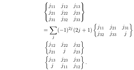
§34.6 Definition: $\mathit{9}j$ Symbol

►The $\mathit{9}j$ symbol may be defined either in terms of $\mathit{3}j$ symbols or equivalently in terms of $\mathit{6}j$ symbols: ►

34.6.1

ⓘ

Defines:

: $\mathit{9}j$ symbol

Symbols:

: $\mathit{3}j$ symbol, $j,j_r$: non-negative integers or non-negative integers plus one half., $r$: nonnegative integer and $s$: integer

Permalink:

http://dlmf.nist.gov/34.6.E1

Encodings:

pMML, png, TeX

See also:

Annotations for §34.6 and Ch.34

►

34.6.2

ⓘ

Symbols:

: $\mathit{9}j$ symbol, : $\mathit{6}j$ symbol and $j,j_r$: non-negative integers or non-negative integers plus one half.

Referenced by:

§34.13

Permalink:

http://dlmf.nist.gov/34.6.E2

Encodings:

pMML, png, TeX

See also:

Annotations for §34.6 and Ch.34

►The $\mathit{9}j$ symbol may also be written as a finite triple sum equivalent to a terminating generalized hypergeometric series of three variables with unit arguments. …

2: 9.13 Generalized Airy Functions

… ►Swanson and Headley (1967) define independent solutions $A_n\left(z\right)$ and $B_n\left(z\right)$ of (9.13.1) by …When $n=1$, $A_n\left(z\right)$ and $B_n\left(z\right)$ become $\mathrm{Ai}\left(z\right)$ and $\mathrm{Bi}\left(z\right)$, respectively. ►Properties of $A_n\left(z\right)$ and $B_n\left(z\right)$ follow from the corresponding properties of the modified Bessel functions. … ►The distribution in $ℂ$ and asymptotic properties of the zeros of $A_n\left(z\right)$, $A_n^{\prime }\left(z\right)$, $B_n\left(z\right)$, and $B_n^{\prime }\left(z\right)$ are investigated in Swanson and Headley (1967) and Headley and Barwell (1975). … ►Their relations to the functions $A_n\left(z\right)$ and $B_n\left(z\right)$ are given by …

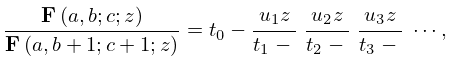
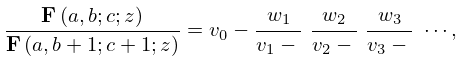
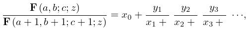
3: 15.7 Continued Fractions

… ►

15.7.1 $$\frac{𝐅(a,b;c;z)}{𝐅(a,b+1;c+1;z)}=t_0-\frac{u_{1}z}{t_1-}\frac{u_{2}z}{t_2-}\frac{u_{3}z}{t_3-}\mathrm{\cdots },$$

ⓘ

Symbols:

$𝐅(a,b;c;z)$ or $𝐅(\genfrac{}{}{0pt}{}{a,b}{c};z)$: $={}_2{}^{}𝐅_1^{}(a,b;c;z)$ Olver’s hypergeometric function, $z$: complex variable, $a$: real or complex parameter, $b$: real or complex parameter, $c$: real or complex parameter, $t_n$: coefficient and $u_n$: coefficient

Permalink:

http://dlmf.nist.gov/15.7.E1

Encodings:

pMML, png, TeX

See also:

Annotations for §15.7 and Ch.15

… ►

15.7.3 $$\frac{𝐅(a,b;c;z)}{𝐅(a,b+1;c+1;z)}=v_0-\frac{w_1}{v_1-}\frac{w_2}{v_2-}\frac{w_3}{v_3-}\mathrm{\cdots },$$

ⓘ

Symbols:

$𝐅(a,b;c;z)$ or $𝐅(\genfrac{}{}{0pt}{}{a,b}{c};z)$: $={}_2{}^{}𝐅_1^{}(a,b;c;z)$ Olver’s hypergeometric function, $z$: complex variable, $a$: real or complex parameter, $b$: real or complex parameter, $c$: real or complex parameter, $v_n$: coefficient and $w_n$: coefficient

Permalink:

http://dlmf.nist.gov/15.7.E3

Encodings:

pMML, png, TeX

See also:

Annotations for §15.7 and Ch.15

… ►

15.7.5 $$\frac{𝐅(a,b;c;z)}{𝐅(a+1,b+1;c+1;z)}=x_0+\frac{y_1}{x_1+}\frac{y_2}{x_2+}\frac{y_3}{x_3+}\mathrm{\cdots },$$

ⓘ

Symbols:

$𝐅(a,b;c;z)$ or $𝐅(\genfrac{}{}{0pt}{}{a,b}{c};z)$: $={}_2{}^{}𝐅_1^{}(a,b;c;z)$ Olver’s hypergeometric function, $x$: real variable, $y$: real variable, $z$: complex variable, $a$: real or complex parameter, $b$: real or complex parameter and $c$: real or complex parameter

Permalink:

http://dlmf.nist.gov/15.7.E5

Encodings:

pMML, png, TeX

See also:

Annotations for §15.7 and Ch.15

…

4: Bibliography I

… ►

Highly Oscillatory Quadrature: The Story So Far. In Numerical Mathematics and Advanced Applications, A. Bermudez de Castro and others (Eds.), pp. 97–118.

ⓘ

Notes:

Proceedings of ENuMath, Santiago de Compostela (2005)

External Links:

ISBN 3-540-34287-7, MathReview, ZentralBlatt

Referenced by:

§3.5(vii).

Encodings:

BibTeX

… ►

Classical and Quantum Orthogonal Polynomials in One Variable. Encyclopedia of Mathematics and its Applications, Vol. 98, Cambridge University Press, Cambridge.

ⓘ

External Links:

ISBN 978-0-521-78201-2; 0-521-78201-5, MathReview Entry, ZentralBlatt

Referenced by:

§1.4(v), Profile Mourad E.H. Ismail, Erratum (V1.0.20) for Chapter 18 Orthogonal Polynomials.

Encodings:

BibTeX

►

Classical and Quantum Orthogonal Polynomials in One Variable. Encyclopedia of Mathematics and its Applications, Vol. 98, Cambridge University Press, Cambridge.

ⓘ

Notes:

With two chapters by Walter Van Assche, With a foreword by Richard A. Askey, Corrected reprint of the 2005 original.

External Links:

ISBN 978-0-521-14347-9, MathReview Entry, ZentralBlatt

Referenced by:

§18.12, (18.15.4_5), (18.16.19), (18.16.20), (18.16.21), §18.17(ii), §18.18(vii), §18.19, (18.2.20), §18.2(vi), §18.2(xii), §18.2(xii), §18.2(x), §18.20(i), §18.20(ii), §18.21(ii), §18.22(i), §18.22(ii), §18.22(iii), §18.23, §18.25(i), §18.25(iii), §18.26(i), §18.26(iv), (18.27.4), §18.27(i), §18.27(ii), §18.27(iii), §18.27(v), §18.27(vi), §18.28(i), §18.28(ii), §18.28(iii), §18.28(v), §18.28(vi), §18.28(vii), §18.28(viii), §18.30(vi), §18.30(vii), §18.30(iii), §18.30(iv), §18.30, §18.30(vi), §18.34(i), §18.34(ii), §18.34(ii), §18.34(iii), (18.35.4), (18.35.5), (18.35.6), (18.35.6_2), (18.35.6_3), (18.35.6_4), (18.35.7), (18.35.8), §18.35(ii), §18.35(iii), §18.36(iii), §18.38(ii), §18.39(iv), §18.39(iv), §18.39(iv), (18.40.4), Profile Mourad E.H. Ismail, Erratum (V1.0.20) for Chapter 18 Orthogonal Polynomials.

Encodings:

BibTeX

…

5: 6.14 Integrals

… ►

6.14.1 $${\int }_0^{\mathrm{\infty }}{\mathrm{e}}^{-at}{E}_1\left(t\right)dt=\frac{1}{a}\ln \left(1+a\right),$$ $\mathrm{\Re }a>-1$,

ⓘ

Symbols:

$dx$: differential of $x$ , $\mathrm{e}$: base of natural logarithm, $E_1\left(z\right)$: exponential integral, $\int$: integral, $\ln z$: principal branch of logarithm function and $\mathrm{\Re }$: real part

A&S Ref:

5.1.34 (special case of)

Permalink:

http://dlmf.nist.gov/6.14.E1

Encodings:

pMML, png, TeX

See also:

Annotations for §6.14(i), §6.14 and Ch.6

… ►

6.14.4 $${\int }_0^{\mathrm{\infty }}{E}_1^2\left(t\right)dt=2\ln 2,$$

ⓘ

Symbols:

$dx$: differential of $x$ , $E_1\left(z\right)$: exponential integral, $\int$: integral and $\ln z$: principal branch of logarithm function

A&S Ref:

5.1.33

Permalink:

http://dlmf.nist.gov/6.14.E4

Encodings:

pMML, png, TeX

See also:

Annotations for §6.14(ii), §6.14 and Ch.6

… ►For collections of integrals, see Apelblat (1983, pp. 110–123), Bierens de Haan (1939, pp. 373–374, 409, 479, 571–572, 637, 664–673, 680–682, 685–697), Erdélyi et al. (1954a, vol. 1, pp. 40–42, 96–98, 177–178, 325), Geller and Ng (1969), Gradshteyn and Ryzhik (2000, §§5.2–5.3 and 6.2–6.27), Marichev (1983, pp. 182–184), Nielsen (1906b), Oberhettinger (1974, pp. 139–141), Oberhettinger (1990, pp. 53–55 and 158–160), Oberhettinger and Badii (1973, pp. 172–179), Prudnikov et al. (1986b, vol. 2, pp. 24–29 and 64–92), Prudnikov et al. (1992a, §§3.4–3.6), Prudnikov et al. (1992b, §§3.4–3.6), and Watrasiewicz (1967).

6: 33.20 Expansions for Small $|ϵ|$

… ►where ►

33.20.4 $${𝖥}_k(\mathrm{\ell };r)=\sum _{p=2k}^{3k}{(2r)}^{(p+1)/2}{C}_{k,p}{J}_{2\mathrm{\ell }+1+p}\left(\sqrt{8r}\right),$$ $r>0$,

ⓘ

Symbols:

$J_{\nu }\left(z\right)$: Bessel function of the first kind, $k$: nonnegative integer, $\mathrm{\ell }$: nonnegative integer, $r$: real variable, ${𝖥}_k(\mathrm{\ell };r)$: coefficient and $C_{k,p}$: coefficients

Permalink:

http://dlmf.nist.gov/33.20.E4

Encodings:

pMML, png, TeX

See also:

Annotations for §33.20(ii), §33.20 and Ch.33

… ►The functions $J$ and $I$ are as in §§10.2(ii), 10.25(ii), and the coefficients $C_{k,p}$ are given by $C_{0,0}=1$, $C_{1,0}=0$, and … ►where $A(ϵ,\mathrm{\ell })$ is given by (33.14.11), (33.14.12), and …The functions $Y$ and $K$ are as in §§10.2(ii), 10.25(ii), and the coefficients $C_{k,p}$ are given by (33.20.6). …

7: Bibliography O

… ►

Summing one- and two-dimensional series related to the Euler series. J. Comput. Appl. Math. 98 (2), pp. 245–271.

ⓘ

External Links:

ISSN 0377-0427, Document, MathReview (Boris Petrovich Osilenker), ZentralBlatt

Referenced by:

§25.8.

Encodings:

BibTeX

… ►

Uniform asymptotic expansions for hypergeometric functions with large parameters. III. Analysis and Applications (Singapore) 8 (2), pp. 199–210.

ⓘ

External Links:

ISSN 0219-5305, Document, MathReview (Javier Segura), ZentralBlatt

Referenced by:

§15.12(iii).

Encodings:

BibTeX

… ►

On an asymptotic expansion of a ratio of gamma functions. Proc. Roy. Irish Acad. Sect. A 95 (1), pp. 5–9.

ⓘ

External Links:

ISSN 0035-8975, MathReview (Richard B. Paris), ZentralBlatt

Referenced by:

§5.11(iii).

Encodings:

BibTeX

… ►

Numerical evaluation of the dilogarithm of complex argument. Celestial Mech. Dynam. Astronom. 62 (1), pp. 93–98.

ⓘ

External Links:

ISSN 0923-2958, Document, MathReview (Bruce C. Berndt), ZentralBlatt

Referenced by:

§25.18(i).

Encodings:

BibTeX

… ►

Solution of Equations in Euclidean and Banach Spaces. Pure and Applied Mathematics, Vol. 9, Academic Press, New York-London.

ⓘ

Notes:

Third edition of Solution of equations and systems of equations

External Links:

MathReview (J. Burlak), ZentralBlatt

Referenced by:

§3.3(v), §3.8(iii).

Encodings:

BibTeX

…

8: 27.2 Functions

… ►

27.2.9 $$d\left(n\right)=\sum _{d|n}1$$

ⓘ

Symbols:

$d_k\left(n\right)$: divisor function, $d$: positive integer and $n$: positive integer

A&S Ref:

24.3.3 I.A

Permalink:

http://dlmf.nist.gov/27.2.E9

Encodings:

pMML, png, TeX

See also:

Annotations for §27.2(i), §27.2 and Ch.27

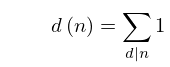
… ►It is the special case $k=2$ of the function $d_k\left(n\right)$ that counts the number of ways of expressing $n$ as the product of $k$ factors, with the order of factors taken into account. …Note that ${\sigma }_0\left(n\right)=d\left(n\right)$. … ►Table 27.2.2 tabulates the Euler totient function $\varphi \left(n\right)$, the divisor function $d\left(n\right)$ ($={\sigma }_0(n)$), and the sum of the divisors $\sigma (n)$ ($={\sigma }_1(n)$), for $n=1(1)52$. … ►

Table 27.2.2: Functions related to division.

► ►►►

$n$	$\varphi \left(n\right)$	$d\left(n\right)$	$\sigma \left(n\right)$	$n$	$\varphi \left(n\right)$	$d\left(n\right)$	$\sigma \left(n\right)$	$n$	$\varphi \left(n\right)$	$d\left(n\right)$	$\sigma \left(n\right)$	$n$	$\varphi \left(n\right)$	$d\left(n\right)$	$\sigma \left(n\right)$
…
13	12	2	14	26	12	4	42	39	24	4	56	52	24	6	98

►

9: Bibliography

… ►

Summations and transformations for basic Appell series. J. London Math. Soc. (2) 4, pp. 618–622.

ⓘ

External Links:

MathReview (R. N. Jain), ZentralBlatt

Referenced by:

§17.11.

Encodings:

BibTeX

… ►

Theorems on generalized Dedekind sums. Pacific J. Math. 2 (1), pp. 1–9.

ⓘ

External Links:

MathReview (N. G. de Bruijn), ZentralBlatt

Referenced by:

(25.11.41), (25.11.42), §25.11(xii).

Encodings:

BibTeX

… ►

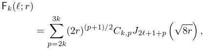
Numerical Tables for Angular Correlation Computations in $\alpha$-, $\beta$- and $\gamma$-Spectroscopy: $3j$-, $6j$-, $9j$-Symbols, F- and $\mathrm{\Gamma }$-Coefficients. Landolt-Börnstein Numerical Data and Functional Relationships in Science and Technology, Springer-Verlag.

ⓘ

External Links:

ISBN 978-3-540-04218-1

Referenced by:

§34.14.

Encodings:

BibTeX

… ►

A new treatment of the ellipsoidal wave equation. Proc. London Math. Soc. (3) 9, pp. 21–50.

ⓘ

External Links:

ISSN 0024-6115, Document, MathReview (J. Meixner), ZentralBlatt

Referenced by:

§29.11.

Encodings:

BibTeX

… ►

Positive Jacobi polynomial sums. II. Amer. J. Math. 98 (3), pp. 709–737.

ⓘ

External Links:

FullText, MathReview (F. Schipp), ZentralBlatt

Referenced by:

§16.23(iii), (18.14.25), (18.14.26), (18.14.27), (18.38.3), Profile Richard A. Askey.

Encodings:

BibTeX

…

10: Bibliography G

… ►

Quasirandom distributed bases for bound problems. J. Chem. Phys. 114 (9), pp. 3929–3939.

ⓘ

Referenced by:

§18.39(iii).

Encodings:

BibTeX

… ►

Algorithm 292: Regular Coulomb wave functions. Comm. ACM 9 (11), pp. 793–795.

ⓘ

External Links:

ISSN 0001-0782, Document

Referenced by:

§33.26(ii).

Encodings:

BibTeX

… ►

Computational aspects of three-term recurrence relations. SIAM Rev. 9 (1), pp. 24–82.

ⓘ

External Links:

Document, MathReview (E. Frank), ZentralBlatt

Referenced by:

§10.74(iv), §14.32, §3.10(iii), §3.6(iii).

Encodings:

BibTeX

… ►

Computational Methods in Special Functions – A Survey. In Theory and Application of Special Functions (Proc. Advanced Sem., Math. Res. Center, Univ. Wisconsin, Madison, Wis., 1975), R. A. Askey (Ed.), pp. 1–98. Math. Res. Center, Univ. Wisconsin Publ., No. 35.

ⓘ

External Links:

MathReview (H. E. Fettis), ZentralBlatt

Referenced by:

§19.36(ii), §19.5.

Encodings:

BibTeX

… ►

Integral representations for computing real parabolic cylinder functions. Numer. Math. 98 (1), pp. 105–134.

ⓘ

External Links:

ISSN 0029-599X, Document, MathReview Entry, ZentralBlatt

Referenced by:

§12.18.

Encodings:

BibTeX

…