.%E5%8E%86%E5%B1%8A%E4%B8%96%E7%95%8C%E6%9D%AF%E9%87%91%E7%90%83%E5%A5%96%E6%95%B0%E9%87%8F%E3%80%8E%E7%BD%91%E5%9D%80%3Amxsty.cc%E3%80%8F.2017%E8%B6%B3%E7%90%83%E4%B8%96%E7%95%8C%E6%9D%AF%E6%AF%94%E8%B5%9B-m6q3s2-2022%E5%B9%B411%E6%9C%8829%E6%97%A56%E6%97%B617%E5%88%8650%E7%A7%92.nzpvd1p5z

♦ 1—10 of 743 matching pages ♦

Did you mean .%E5%8E%86%E5%B1%8A%E4%B8%96%E7%95%8C%E6%9D%AF%E9%87%91%E7%90%83%E5%A5%96%E6%95%B0%E9%87%8F%E3%80%8E%E7%BD%91%E5%9D%80%3Amxsty.cc%E3%80%8F.2017%E8%B6%B3%E7%90%83%E4%B8%96%E7%95%8C%E6%9D%AF%E6%AF%94%E8%B5%9B-m6q3s2-2022%E5%B9%411%E6%9C%882%E6%97%256%E6%97%617%E5%88%865%E7%A7%92.nzpvd1p5z ?

(0.042 seconds)

1—10 of 743 matching pages

1: 8 Incomplete Gamma and Related
Functions

Chapter 8 Incomplete Gamma and Related Functions

…

2: 8.19 Generalized Exponential Integral

… ►Most properties of

E_{p}\left(z\right)

follow straightforwardly from those of

\Gamma\left(a,z\right)

. For an extensive treatment of

E_{1}\left(z\right)

see Chapter 6. … ►Integral representations of Mellin–Barnes type for

E_{p}\left(z\right)

follow immediately from (8.6.11), (8.6.12), and (8.19.1). … ►The general function

E_{p}\left(z\right)

is attained by extending the path in (8.19.2) across the negative real axis. Unless

p

is a nonpositive integer,

E_{p}\left(z\right)

has a branch point at

z=0

. …

3: 24.2 Definitions and Generating Functions

… ►

E_{2n+1}=0

… ►

24.2.9

E_{n}=2^{n}E_{n}\left(\tfrac{1}{2}\right)=\text{integer},

ⓘ

Symbols:: $E_{\NVar{n}}$ : Euler numbers, $E_{\NVar{n}}\left(\NVar{x}\right)$ : Euler polynomials and $n$ : integer
A&S Ref:: 23.1.2
Permalink:: http://dlmf.nist.gov/24.2.E9
Encodings:: pMML, png, TeX
See also:: Annotations for §24.2(ii), §24.2 and Ch.24

… ►

\widetilde{E}_{n}\left(x\right)=E_{n}\left(x\right)

0\leq x<1

… ►

\widetilde{E}_{n}\left(x+1\right)=-\widetilde{E}_{n}\left(x\right)

x\in\mathbb{R}

… ►

Table 24.2.4: Euler numbers

E_{n}

► ►►

$n$	$E_{n}$
…

► …

4: 8.20 Asymptotic Expansions of $E_{p}\left(z\right)$

§8.20 Asymptotic Expansions of $E_{p}\left(z\right)$

… ►For an exponentially-improved asymptotic expansion of

E_{p}\left(z\right)

see §2.11(iii). … ►For

x\geq 0

and

p>1

let

x=\lambda p

and define

A_{0}(\lambda)=1

, …so that

A_{k}(\lambda)

is a polynomial in

\lambda

of degree

k-1

when

k\geq 1

. … ►

A_{3}(\lambda)=1-8\lambda+6\lambda^{2}.

…

5: 3.1 Arithmetics and Error Measures

… ►with

b_{0}=1

and all allowable choices of

E

p

s

, and

b_{j}

. … ►Let

E_{{\rm min}}\leq E\leq E_{{\rm max}}

with

E_{{\rm min}}<0

and

E_{{\rm max}}>0

. For given values of

E_{{\rm min}}

E_{{\rm max}}

, and

p

, the format width in bits

N

of a computer word is the total number of bits: the sign (one bit), the significant bits

b_{1},b_{2},\dots,b_{p-1}

(

p-1

bits), and the bits allocated to the exponent (the remaining

N-p

bits). The integers

p

E_{{\rm min}}

, and

E_{{\rm max}}

are characteristics of the machine. … ►In the case of the normalized binary interchange formats, the representation of data for binary32 (previously single precision) (

N=32

p=24

E_{{\rm min}}=-126

E_{{\rm max}}=127

), binary64 (previously double precision) (

N=64

p=53

E_{{\rm min}}=-1022

E_{{\rm max}}=1023

) and binary128 (previously quad precision) (

N=128

p=113

E_{{\rm min}}=-16382

E_{{\rm max}}=16383

) are as in Figure 3.1.1. …

6: 6.20 Approximations

… ►

•

Hastings (1955) gives several minimax polynomial and rational approximations for $E_{1}\left(x\right)+\ln x$ , $xe^{x}E_{1}\left(x\right)$ , and the auxiliary functions $\mathrm{f}\left(x\right)$ and $\mathrm{g}\left(x\right)$ . These are included in Abramowitz and Stegun (1964, Ch. 5).

►

•

Cody and Thacher (1968) provides minimax rational approximations for $E_{1}\left(x\right)$ , with accuracies up to 20S.

… ►

•

Clenshaw (1962) gives Chebyshev coefficients for $-E_{1}\left(x\right)-\ln|x|$ for $-4\leq x\leq 4$ and $e^{x}E_{1}\left(x\right)$ for $x\geq 4$ (20D).

… ►

•

Luke (1969b, pp. 321–322) covers $\operatorname{Ein}\left(x\right)$ and $-\operatorname{Ein}\left(-x\right)$ for $0\leq x\leq 8$ (the Chebyshev coefficients are given to 20D); $E_{1}\left(x\right)$ for $x\geq 5$ (20D), and $\operatorname{Ei}\left(x\right)$ for $x\geq 8$ (15D). Coefficients for the sine and cosine integrals are given on pp. 325–327.

… ►

•

Luke (1969b, pp. 402, 410, and 415–421) gives main diagonal Padé approximations for $\operatorname{Ein}\left(z\right)$ , $\operatorname{Si}\left(z\right)$ , $\operatorname{Cin}\left(z\right)$ (valid near the origin), and $E_{1}\left(z\right)$ (valid for large $|z|$ ); approximate errors are given for a selection of $z$ -values.

…

7: 11.10 Anger–Weber Functions

… ►The Anger function

\mathbf{J}_{\nu}\left(z\right)

and Weber function

\mathbf{E}_{\nu}\left(z\right)

are defined by … ►The associated Anger–Weber function

\mathbf{A}_{\nu}\left(z\right)

is defined by … ►where …For the Fresnel integrals

C

and

S

see §7.2(iii). … ►For

n=1,2,3,\dots

, …

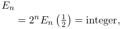
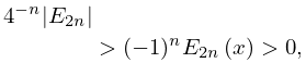
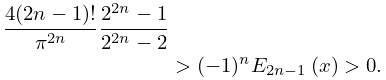
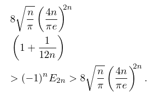
8: 24.9 Inequalities

… ►

24.9.3

4^{-n}|E_{2n}|>(-1)^{n}E_{2n}\left(x\right)>0,

ⓘ

Symbols:: $E_{\NVar{n}}$ : Euler numbers, $E_{\NVar{n}}\left(\NVar{x}\right)$ : Euler polynomials, $n$ : integer and $x$ : real or complex
A&S Ref:: 23.1.13
Referenced by:: §24.9, §24.9
Permalink:: http://dlmf.nist.gov/24.9.E3
Encodings:: pMML, png, TeX
See also:: Annotations for §24.9 and Ch.24

… ►

24.9.5

\frac{4(2n-1)!}{\pi^{2n}}\frac{2^{2n}-1}{2^{2n}-2}>(-1)^{n}E_{2n-1}\left(x% \right)>0.

ⓘ

Symbols:: $E_{\NVar{n}}\left(\NVar{x}\right)$ : Euler polynomials, $\pi$ : the ratio of the circumference of a circle to its diameter, $!$ : factorial (as in $n!$ ), $n$ : integer and $x$ : real or complex
A&S Ref:: 23.1.14
Referenced by:: §24.9, §24.9
Permalink:: http://dlmf.nist.gov/24.9.E5
Encodings:: pMML, png, TeX
See also:: Annotations for §24.9 and Ch.24

►(24.9.6)–(24.9.7) hold for

n=2,3,\dotsc

. … ►

24.9.7

8\sqrt{\frac{n}{\pi}}\left(\frac{4n}{\pi e}\right)^{2n}\left(1+\frac{1}{12n}% \right)>(-1)^{n}E_{2n}>8\sqrt{\frac{n}{\pi}}\left(\frac{4n}{\pi e}\right)^{2n}.

ⓘ

Symbols:: $E_{\NVar{n}}$ : Euler numbers, $\pi$ : the ratio of the circumference of a circle to its diameter, $\mathrm{e}$ : base of natural logarithm and $n$ : integer
Referenced by:: §24.9, §24.9
Permalink:: http://dlmf.nist.gov/24.9.E7
Encodings:: pMML, png, TeX
See also:: Annotations for §24.9 and Ch.24

… ►

24.9.10

\frac{4^{n+1}(2n)!}{\pi^{2n+1}}>(-1)^{n}E_{2n}>\frac{4^{n+1}(2n)!}{\pi^{2n+1}}% \frac{1}{1+3^{-1-2n}}.

ⓘ

Symbols:: $E_{\NVar{n}}$ : Euler numbers, $\pi$ : the ratio of the circumference of a circle to its diameter, $!$ : factorial (as in $n!$ ) and $n$ : integer
A&S Ref:: 23.1.15
Referenced by:: §24.9
Permalink:: http://dlmf.nist.gov/24.9.E10
Encodings:: pMML, png, TeX
See also:: Annotations for §24.9 and Ch.24

9: 29.17 Other Solutions

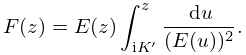
… ►If (29.2.1) admits a Lamé polynomial solution

E

, then a second linearly independent solution

F

is given by ►

29.17.1

F(z)=E(z)\int_{\mathrm{i}{K^{\prime}}}^{z}\frac{\,\mathrm{d}u}{(E(u))^{2}}.

ⓘ

Symbols:: ${K^{\prime}}\left(\NVar{k}\right)$ : Legendre’s complementary complete elliptic integral of the first kind, $\,\mathrm{d}\NVar{x}$ : differential of $x$ , $\mathrm{i}$ : imaginary unit, $\int$ : integral, $z$ : complex variable and $k$ : real parameter
Permalink:: http://dlmf.nist.gov/29.17.E1
Encodings:: pMML, png, TeX
See also:: Annotations for §29.17(i), §29.17 and Ch.29

… ►They are algebraic functions of

\operatorname{sn}\left(z,k\right)

\operatorname{cn}\left(z,k\right)

, and

\operatorname{dn}\left(z,k\right)

, and have primitive period

8K

. …

10: 24.20 Tables

… ►Wagstaff (1978) gives complete prime factorizations of

N_{n}

and

E_{n}

for

n=20(2)60

and

n=8(2)42

, respectively. In Wagstaff (2002) these results are extended to

n=60(2)152

and

n=40(2)88

, respectively, with further complete and partial factorizations listed up to

n=300

and

n=200

, respectively. …

.%E5%8E%86%E5%B1%8A%E4%B8%96%E7%95%8C%E6%9D%AF%E9%87%91%E7%90%83%E5%A5%96%E6%95%B0%E9%87%8F%E3%80%8E%E7%BD%91%E5%9D%80%3Amxsty.cc%E3%80%8F.2017%E8%B6%B3%E7%90%83%E4%B8%96%E7%95%8C%E6%9D%AF%E6%AF%94%E8%B5%9B-m6q3s2-2022%E5%B9%B411%E6%9C%8829%E6%97%A56%E6%97%B617%E5%88%8650%E7%A7%92.nzpvd1p5z

1—10 of 743 matching pages

1: 8 Incomplete Gamma and Related Functions

Chapter 8 Incomplete Gamma and Related Functions

2: 8.19 Generalized Exponential Integral

3: 24.2 Definitions and Generating Functions

4: 8.20 Asymptotic Expansions of E p ⁡ ( z )

§8.20 Asymptotic Expansions of E p ⁡ ( z )

5: 3.1 Arithmetics and Error Measures

6: 6.20 Approximations

7: 11.10 Anger–Weber Functions

8: 24.9 Inequalities

9: 29.17 Other Solutions

10: 24.20 Tables

1: 8 Incomplete Gamma and Related
Functions

4: 8.20 Asymptotic Expansions of $E_{p}\left(z\right)$

§8.20 Asymptotic Expansions of $E_{p}\left(z\right)$